Black-Scholes as the heat equation

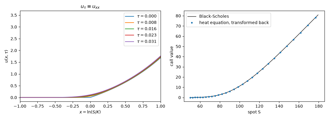
Black and Scholes (1973) found their formula by changing variables until the pricing equation became the heat equation. With \(x = \ln(S/K)\) and \(\tau = \tfrac12\sigma^2(T - t)\), \(V = K e^{\alpha x + \beta\tau} u\) turns Black-Scholes into \(u_\tau = u_{xx}\), whose initial condition is the transformed payoff. heat_equation_price() solves the heat equation by Crank-Nicolson on a uniform grid, watches the payoff diffuse, and transforms back.

import matplotlib.pyplot as plt

from financialkit.options import black_scholes_price
from financialkit.pde_methods import heat_equation_price
from financialkit.pde_methods.visualizers import plot_heat_solution

S, K, T, r, sigma, q = 100.0, 100.0, 1.0, 0.05, 0.25, 0.02
res = heat_equation_price(S, K, T, r, sigma, q, n_space=400, n_time=100)
print(f"alpha = {res.alpha:.3f}, beta = {res.beta:.3f}, tau_end = {res.tau[-1]:.4f}")
print(f"heat equation {res.price:.5f}, Black-Scholes {black_scholes_price(S, K, T, r, sigma, q):.5f}")

alpha = 0.020, beta = -1.600, tau_end = 0.0312
heat equation 11.12264, Black-Scholes 11.12376

The payoff diffusing in heat-equation variables, and back in prices

fig, axes = plt.subplots(1, 2, figsize=(11, 4))
plot_heat_solution(res, n_curves=5, ax=axes[0])
axes[0].set_xlim(-1.0, 1.0)
axes[0].set_title(r"$u_\tau = u_{xx}$")

near = (res.S > 50) & (res.S < 180)
axes[1].plot(res.S[near], black_scholes_price(res.S[near], K, T, r, sigma, q), "k", lw=1, label="Black-Scholes")
axes[1].plot(res.S[near][::6], res.V[near][::6], "o", ms=3, label="heat equation, transformed back")
axes[1].set_xlabel("spot S")
axes[1].set_ylabel("call value")
axes[1].legend()
fig.tight_layout()
plt.show()