The Thomas algorithm

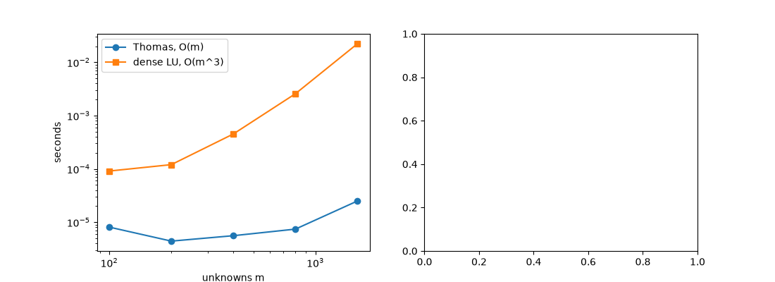
Every implicit step in one space dimension is a tridiagonal system. Llewellyn Thomas (1949) wrote down the specialised Gaussian elimination that solves it in \(O(m)\) operations: one sweep removes the sub-diagonal, a second substitutes back. No pivoting is needed because the implicit Black-Scholes matrix is diagonally dominant. thomas_solve() is that algorithm by hand; it agrees with scipy.linalg.solve_banded() to rounding, and its cost grows linearly while a dense solve grows cubically.

import time

import matplotlib.pyplot as plt
import numpy as np

from financialkit.pde_methods import CrankNicolson, black_scholes_operator, solve_tridiagonal, thomas_solve, tridiagonal_matrix

# One implicit step's matrix, I - dt A, on a 200-interval grid
S = np.linspace(0.0, 400.0, 201)
lower, diag, upper = black_scholes_operator(S, 0.2, 0.05)
dt = 0.01
lo, di, up = -dt * lower, 1.0 - dt * diag, -dt * upper
rhs = np.maximum(S[1:-1] - 100.0, 0.0)

x = thomas_solve(lo, di, up, rhs)
print("max |Thomas - solve_banded| =", np.abs(x - solve_tridiagonal(lo, di, up, rhs)).max())
print("diagonally dominant:", bool(np.all(np.abs(di) >= np.abs(lo) + np.abs(up))))

max |Thomas - solve_banded| = 1.7053025658242404e-13
diagonally dominant: True

Linear against cubic cost

sizes = np.array([100, 200, 400, 800, 1600])
t_thomas, t_dense = [], []
for m in sizes:
    lo_m, up_m = np.full(m, -1.0), np.full(m, -1.0)
    di_m, b = np.full(m, 2.5), np.ones(m)
    dense = tridiagonal_matrix(lo_m, di_m, up_m).toarray()
    t0 = time.perf_counter()
    thomas_solve(lo_m, di_m, up_m, b)
    t_thomas.append(time.perf_counter() - t0)
    t0 = time.perf_counter()
    np.linalg.solve(dense, b)
    t_dense.append(time.perf_counter() - t0)

fig, axes = plt.subplots(1, 2, figsize=(11, 4))
axes[0].loglog(sizes, t_thomas, "o-", label="Thomas, O(m)")
axes[0].loglog(sizes, t_dense, "s-", label="dense LU, O(m^3)")
axes[0].set_xlabel("unknowns m")
axes[0].set_ylabel("seconds")
axes[0].legend()

<matplotlib.legend.Legend object at 0x116c09e80>

The same prices from either solver

a = CrankNicolson(200, 50, solver="thomas").price(100.0, 100.0, 1.0, 0.05, 0.2)
b = CrankNicolson(200, 50, solver="banded").price(100.0, 100.0, 1.0, 0.05, 0.2)
axes[1].semilogy(a.S, np.abs(a.V - b.V) + 1e-18)
axes[1].set_xlabel("spot S")
axes[1].set_title("|Thomas - solve_banded| over the grid")
fig.tight_layout()
plt.show()