Truth in Lending: APR and the effective rate

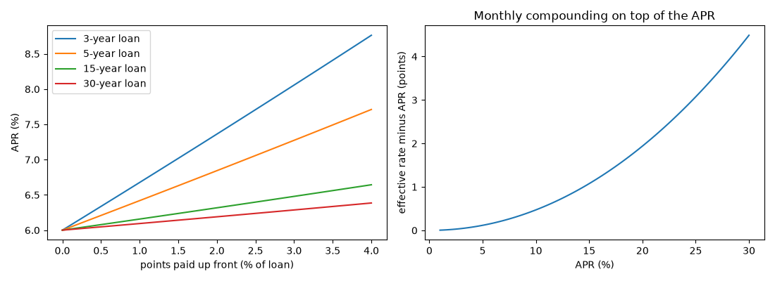
The U.S. Truth in Lending Act (1968) and its Regulation Z made lenders disclose an annual percentage rate computed one way for everyone: the nominal rate at which the payments are worth exactly the amount the borrower actually receives, after fees and points. The APR therefore rises above the note rate when fees are charged, and the faster the loan is repaid, the more the fees count. The APR is still a nominal rate; compounded monthly, the effective annual rate is higher again.

import matplotlib.pyplot as plt
import numpy as np

from financialkit.time_value import annual_percentage_rate, effective_annual_rate, loan_payment

A 200,000 mortgage at 6% with two points

payment = loan_payment(200_000.0, 0.06, 360)
apr = annual_percentage_rate(200_000.0 - 4_000.0, payment, 360)
print(f"note rate 6.000%, APR {apr:.3%}, effective annual rate {effective_annual_rate(apr, 12):.3%}")

note rate 6.000%, APR 6.189%, effective annual rate 6.368%

Fees weigh more on short loans

points = np.linspace(0.0, 4.0, 41)
fig, axes = plt.subplots(1, 2, figsize=(11, 4))
for years in (3, 5, 15, 30):
    n = 12 * years
    p = loan_payment(200_000.0, 0.06, n)
    aprs = [annual_percentage_rate(200_000.0 * (1 - pt / 100), p, n) for pt in points]
    axes[0].plot(points, 100 * np.array(aprs), label=f"{years}-year loan")
axes[0].set_xlabel("points paid up front (% of loan)")
axes[0].set_ylabel("APR (%)")
axes[0].legend()

rates = np.linspace(0.01, 0.30, 100)
axes[1].plot(100 * rates, 100 * (effective_annual_rate(rates, 12) - rates))
axes[1].set_xlabel("APR (%)")
axes[1].set_ylabel("effective rate minus APR (points)")
axes[1].set_title("Monthly compounding on top of the APR")
fig.tight_layout()

plt.show()