Baldwin’s modified IRR

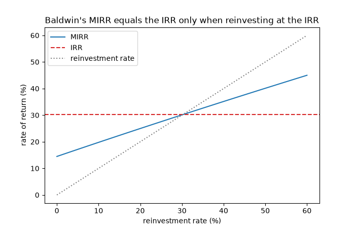
Robert Baldwin’s “How to Assess Investment Proposals” (Harvard Business Review, 1959) proposed a fix for the IRR’s two defects – multiple roots and the implicit assumption that interim cash flows are reinvested at the IRR itself. Compound the inflows to the horizon at a realistic reinvestment rate, discount the outflows at the finance rate, and report the one rate that links them: \(\mathrm{MIRR} = (FV^+ / |PV^-|)^{1/n} - 1\). It always exists and is unique.

import matplotlib.pyplot as plt
import numpy as np

from financialkit.time_value import irr, irr_all, mirr

A high-IRR project

Its IRR assumes the early inflows earn the IRR again; at a 10% reinvestment rate the realistic return is much lower.

cf = [-1000.0, 800.0, 500.0, 200.0]
print(f"IRR  = {irr(cf):.2%}")
print(f"MIRR = {mirr(cf, 0.10, 0.10):.2%} (finance and reinvest at 10%)")

IRR  = 30.20%
MIRR = 19.77% (finance and reinvest at 10%)

The pump problem gets one answer

pump = [-1600.0, 10_000.0, -10_000.0]
print(f"pump IRRs: {irr_all(pump)}; MIRR at 10%: {mirr(pump, 0.10, 0.10):.2%}")

pump IRRs: [0.25 4.  ]; MIRR at 10%: 5.60%

MIRR moves between the reinvestment rate and the IRR

reinvest = np.linspace(0.0, 0.6, 121)
fig, ax = plt.subplots(figsize=(7, 4.5))
ax.plot(100 * reinvest, [100 * mirr(cf, 0.10, r) for r in reinvest], label="MIRR")
ax.axhline(100 * irr(cf), color="tab:red", ls="--", label="IRR")
ax.plot(100 * reinvest, 100 * reinvest, ":", color="gray", label="reinvestment rate")
ax.set_xlabel("reinvestment rate (%)")
ax.set_ylabel("rate of return (%)")
ax.set_title("Baldwin's MIRR equals the IRR only when reinvesting at the IRR")
ax.legend()

plt.show()