Buchberger’s algorithm for Gröbner bases

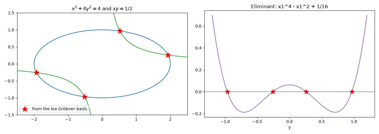
Gaussian elimination solves linear systems by making them triangular. Buchberger’s 1965 thesis did the same for systems of polynomial equations: complete the generators to a Gröbner basis, adding the remainder of every S-polynomial (a combination in which two leading terms cancel) until all of them reduce to zero. With a lexicographic order the basis is triangular: its last element involves only the last variable, so the system is solved by one-variable root finding and back substitution.

import matplotlib.pyplot as plt
import numpy as np

from mathematicskit.abstract_algebra import MultivariatePolynomial, groebner_basis, in_ideal, multivariate_divide

x, y = MultivariatePolynomial.variables(2)

Where an ellipse meets a hyperbola

f = x**2 + 4 * y**2 - 4  # ellipse
g = x * y - MultivariatePolynomial({(0, 0): "1/2"}, 2)  # hyperbola xy = 1/2
result = groebner_basis([f, g], "lex")
print(f"lex Gröbner basis ({result.s_pairs} S-polynomials, {result.zero_reductions} reduced to zero):")
for p in result.basis:
    print(f"   {p}")

eliminant = result.basis[-1]  # a polynomial in y alone
coefficients = [float(eliminant.terms.get((0, k), 0)) for k in range(eliminant.total_degree, -1, -1)]
y_roots = np.sort(np.roots(coefficients).real)
x_of_y = result.basis[0]  # x + (polynomial in y), from the triangular structure
solutions = [(float(-sum(c * yr ** e[1] for e, c in x_of_y.terms.items() if e[0] == 0)), yr) for yr in y_roots]
for xs, ys in solutions:
    print(f"   solution ({xs:+.6f}, {ys:+.6f}): residuals {xs**2 + 4 * ys**2 - 4:+.1e}, {xs * ys - 0.5:+.1e}")

lex Gröbner basis (4 S-polynomials, 2 reduced to zero):
   8*x1^3 + x0 - 8*x1
   x1^4 - x1^2 + 1/16
   solution (-0.517638, -0.965926): residuals +0.0e+00, +7.8e-16
   solution (-1.931852, -0.258819): residuals +2.7e-15, +3.3e-16
   solution (+1.931852, +0.258819): residuals +8.9e-16, +1.1e-16
   solution (+0.517638, +0.965926): residuals -5.8e-15, -1.1e-14

Division needs a Gröbner basis to be well defined

Dividing by the original generators, the remainder depends on their order, and a member of the ideal can leave a nonzero remainder. By a Gröbner basis, the remainder is unique, and zero exactly for members.

member = (x + y) * f + (y**2 - 3) * g
for divisors, name in (([f, g], "[f, g]"), ([g, f], "[g, f]"), (result.basis, "Gröbner basis")):
    print(f"remainder of (x + y) f + (y^2 - 3) g on division by {name:13s}: {multivariate_divide(member, divisors, 'lex')[1]}")
print(f"in the ideal: {in_ideal(member, result)}; x^2 + y^2 in the ideal: {in_ideal(x**2 + y**2, result)}")

remainder of (x + y) f + (y^2 - 3) g on division by [f, g]       : 0
remainder of (x + y) f + (y^2 - 3) g on division by [g, f]       : 4*x1^3 + 1/2*x0 - 4*x1
remainder of (x + y) f + (y^2 - 3) g on division by Gröbner basis: 0
in the ideal: True; x^2 + y^2 in the ideal: False

The curves and their four intersections

grid_x, grid_y = np.meshgrid(np.linspace(-2.5, 2.5, 400), np.linspace(-1.5, 1.5, 400))
fig, (ax0, ax1) = plt.subplots(1, 2, figsize=(13, 4.6))
ax0.contour(grid_x, grid_y, grid_x**2 + 4 * grid_y**2 - 4, levels=[0], colors="tab:blue")
ax0.contour(grid_x, grid_y, grid_x * grid_y - 0.5, levels=[0], colors="tab:green")
ax0.plot(*np.array(solutions).T, "r*", ms=14, label="from the lex Gröbner basis")
ax0.set_aspect("equal")
ax0.set_title(r"$x^2 + 4y^2 = 4$ and $xy = 1/2$")
ax0.legend(loc="lower left")

ys = np.linspace(-1.2, 1.2, 400)
ax1.plot(ys, np.polyval(coefficients, ys), color="tab:purple")
ax1.axhline(0, color="0.6")
ax1.plot(y_roots, np.zeros_like(y_roots), "r*", ms=12)
ax1.set_xlabel("y")
ax1.set_title(f"Eliminant: {eliminant}")
fig.tight_layout()

The order changes the basis

The ideal has a different reduced basis for each monomial order. Graded orders keep degrees low, and are usually much faster to compute; lex is the one that eliminates variables.

for order in ("lex", "grlex", "grevlex"):
    basis = groebner_basis([f, g], order).basis
    print(f"{order:8s}: {len(basis)} elements, max degree {max(p.total_degree for p in basis)}")

plt.show()

lex     : 2 elements, max degree 4
grlex   : 3 elements, max degree 3
grevlex : 3 elements, max degree 3