Richardson extrapolation: cancelling error terms at a fixed step

Richardson’s idea: if an estimate \(D(h)\) has error \(c_1 h^2 + c_2 h^4 + \dots\), then combining \(D(h)\) and \(D(h/2)\) as \((4D(h/2) - D(h))/3\) cancels the \(h^2\) term. Repeating the combination on successively halved steps removes one error order per level. This example applies richardson_extrapolation() to a central difference and shows it reaching near machine precision from a coarse starting step, where no plain difference quotient can.

import matplotlib.pyplot as plt
import numpy as np

from mathematicskit.calculus import central_difference, richardson_extrapolation

f = np.exp
x0 = 1.0
exact = np.exp(1.0)

One extrapolation step by hand

Two central differences, each only \(O(h^2)\), combine into an \(O(h^4)\) estimate at no extra cost.

h = 0.2
d_h = central_difference(f, x0, h)
d_h2 = central_difference(f, x0, h / 2)
combined = (4 * d_h2 - d_h) / 3
print(f"D(h)   error: {abs(d_h - exact):.3e}")
print(f"D(h/2) error: {abs(d_h2 - exact):.3e}")
print(f"(4D(h/2) - D(h))/3 error: {abs(combined - exact):.3e}")

D(h)   error: 1.816e-02
D(h/2) error: 4.533e-03
(4D(h/2) - D(h))/3 error: 9.072e-06

Each level cancels one more error order

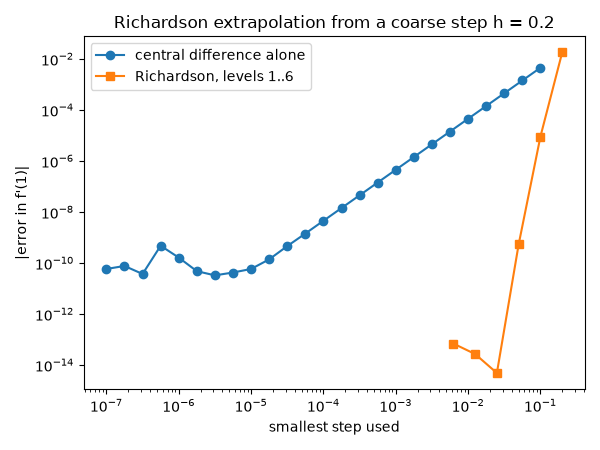
Starting from the same coarse \(h = 0.2\), every extra level of extrapolation gains roughly two more orders of accuracy, until floating-point round-off takes over.

levels = np.arange(1, 7)
errs = [abs(richardson_extrapolation(f, x0, h=0.2, levels=int(k)).value - exact) for k in levels]
for k, e in zip(levels, errs):
    print(f"levels={k}: error={e:.3e}")

levels=1: error=1.816e-02
levels=2: error=9.072e-06
levels=3: error=5.397e-10
levels=4: error=4.885e-15
levels=5: error=2.709e-14
levels=6: error=6.972e-14

Extrapolation beats simply shrinking the step

A plain central difference at step \(h\) bottoms out near \(10^{-11}\) because of cancellation; Richardson reaches that accuracy while its smallest step is still large.

hs = np.logspace(-1, -7, 25)
err_ctr = [abs(central_difference(f, x0, hh) - exact) for hh in hs]
smallest_step = [0.2 / 2 ** (k - 1) for k in levels]

fig, ax = plt.subplots(figsize=(6, 4.5))
ax.loglog(hs, err_ctr, "o-", label="central difference alone")
ax.loglog(smallest_step, np.maximum(errs, 1e-17), "s-", label="Richardson, levels 1..6")
ax.set_xlabel("smallest step used")
ax.set_ylabel("|error in f'(1)|")
ax.set_title("Richardson extrapolation from a coarse step h = 0.2")
ax.legend()
fig.tight_layout()

plt.show()