Newton and Leibniz: the derivative and the integral as limits

The calculus of Newton and Leibniz rests on two limits: the derivative \(dy/dx\) is the limit of a difference quotient, and the integral \(\int f\,dx\) is the limit of a sum of thin strips. This example watches secant slopes (via central_difference()) close in on the tangent slope, and trapezoidal sums (via TrapezoidalRule) close in on the area under the curve – and then checks that the two operations undo each other, as the fundamental theorem of calculus says they must.

import matplotlib.pyplot as plt
import numpy as np

from mathematicskit.calculus import TrapezoidalRule, central_difference

f = np.sin
x0 = 1.0

The derivative: secants become the tangent

Each secant through \(x_0 \pm h\) has slope equal to the central difference quotient; as \(h \to 0\) it turns into the tangent line, whose slope is \(\cos x_0\).

grid = np.linspace(-0.5, 2.5, 400)
fig, (ax1, ax2) = plt.subplots(1, 2, figsize=(10, 4))
ax1.plot(grid, f(grid), "k", lw=2, label=r"$y = \sin x$")
for h in (1.0, 0.5, 0.25):
    slope = central_difference(f, x0, h)
    ax1.plot(grid, f(x0) + slope * (grid - x0), "--", label=f"secant, h={h}")
ax1.plot(grid, f(x0) + np.cos(x0) * (grid - x0), "r", label="tangent")
ax1.plot(x0, f(x0), "ko")
ax1.set_ylim(-1.2, 1.8)
ax1.set_title("dy/dx as a limiting difference quotient")
ax1.legend(fontsize=8)

hs = np.logspace(0, -4, 12)
slope_err = [abs(central_difference(f, x0, h) - np.cos(x0)) for h in hs]
ax2.loglog(hs, slope_err, "o-")
ax2.set_xlabel("h")
ax2.set_ylabel("|secant slope - cos(1)|")
ax2.set_title("the quotient converges as h shrinks")
fig.tight_layout()

for h in (1.0, 0.1, 0.01, 0.001):
    print(f"h={h:<6}: quotient={central_difference(f, x0, h):.10f}  (cos 1 = {np.cos(x0):.10f})")

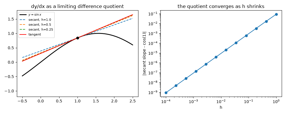
h=1.0   : quotient=0.4546487134  (cos 1 = 0.5403023059)
h=0.1   : quotient=0.5394022522  (cos 1 = 0.5403023059)
h=0.01  : quotient=0.5402933009  (cos 1 = 0.5403023059)
h=0.001 : quotient=0.5403022158  (cos 1 = 0.5403023059)

The integral: strips become the area

Summing \(n\) trapezoidal strips approximates \(\int_0^\pi \sin x\,dx = 2\), and the sum tends to that area as the strips get thinner.

a, b = 0.0, np.pi
fig, (ax1, ax2) = plt.subplots(1, 2, figsize=(10, 4))
fine = np.linspace(a, b, 400)
ax1.plot(fine, f(fine), "k", lw=2)
nodes = np.linspace(a, b, 5)
for left, right in zip(nodes[:-1], nodes[1:]):
    ax1.fill([left, left, right, right], [0, f(left), f(right), 0], alpha=0.3, edgecolor="C0")
ax1.set_title("the integral as a limiting sum (4 strips shown)")

ns = [2, 4, 8, 16, 32, 64, 128]
area_err = [abs(TrapezoidalRule(n=n).integrate(f, a, b).value - 2.0) for n in ns]
ax2.loglog(ns, area_err, "s-")
ax2.set_xlabel("number of strips n")
ax2.set_ylabel("|sum - 2|")
ax2.set_title("the sum converges as the strips thin")
fig.tight_layout()

for n in (4, 16, 64, 256):
    print(f"n={n:<4}: sum of strips={TrapezoidalRule(n=n).integrate(f, a, b).value:.10f}  (exact 2)")

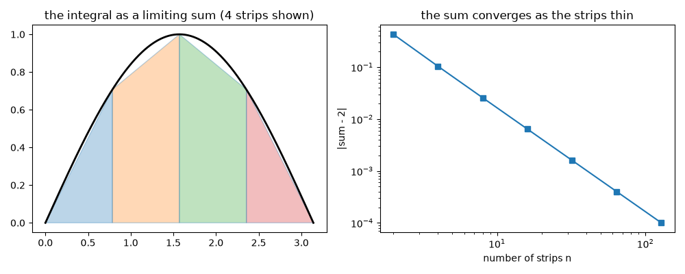
n=4   : sum of strips=1.8961188979  (exact 2)
n=16  : sum of strips=1.9935703438  (exact 2)
n=64  : sum of strips=1.9995983886  (exact 2)
n=256 : sum of strips=1.9999749002  (exact 2)

The two limits are inverse operations

Integrate \(\sin\) from 0 to \(x\), then differentiate the result: the fundamental theorem says we should recover \(\sin x\) itself.

def area_up_to(x):
    return TrapezoidalRule(n=2000).integrate(f, 0.0, x).value


for x in (0.5, 1.0, 2.0):
    recovered = central_difference(area_up_to, x, 1e-3)
    print(f"d/dx of area up to x={x}: {recovered:.6f}  vs  sin(x) = {np.sin(x):.6f}")

plt.show()

d/dx of area up to x=0.5: 0.479425  vs  sin(x) = 0.479426
d/dx of area up to x=1.0: 0.841471  vs  sin(x) = 0.841471
d/dx of area up to x=2.0: 0.909297  vs  sin(x) = 0.909297