Riemann sums: the definition of the integral

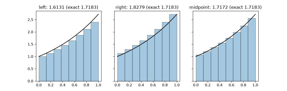
Draws left, right, and midpoint Riemann sums for the same integrand and shows their convergence: first order for the endpoint rules, second order for the midpoint rule.

import matplotlib.pyplot as plt
import numpy as np

from mathematicskit.calculus import RiemannSum
from mathematicskit.calculus.visualizers.plots import plot_quadrature_convergence

Three ways to sample each subinterval

f, a, b, n = np.exp, 0.0, 1.0, 8
exact = np.e - 1
fig, axes = plt.subplots(1, 3, figsize=(11, 3.5), sharey=True)
grid = np.linspace(a, b, 200)
h = (b - a) / n
for ax, rule, offset in zip(axes, ("left", "right", "midpoint"), (0.0, 1.0, 0.5)):
    ax.plot(grid, f(grid), "k")
    left_edges = a + h * np.arange(n)
    ax.bar(left_edges, f(left_edges + offset * h), width=h, align="edge", alpha=0.4, edgecolor="k")
    value = RiemannSum(n, rule).integrate(f, a, b).value
    ax.set_title(f"{rule}: {value:.4f} (exact {exact:.4f})")

Convergence orders

ns = [4, 8, 16, 32, 64, 128, 256]
ax = None
for rule in ("left", "right", "midpoint"):
    ax = plot_quadrature_convergence(lambda n, r=rule: RiemannSum(n, r), f, a, b, exact, ns, ax=ax, label=rule)
ax.set_title("Riemann sums: O(h) at the endpoints, O(h^2) at midpoints")

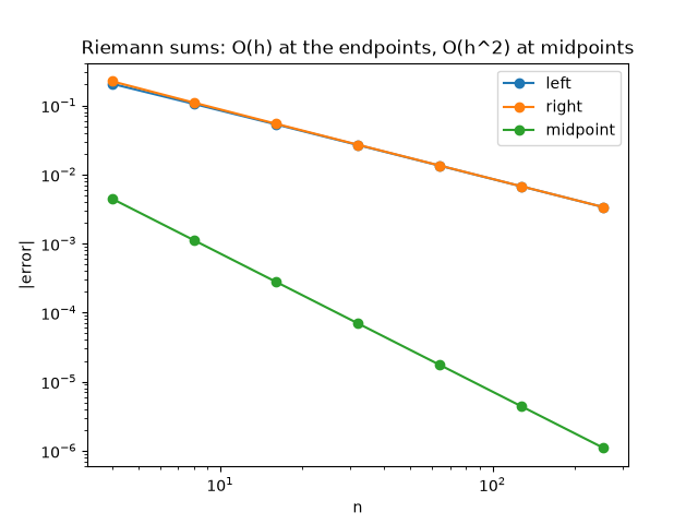
Text(0.5, 1.0, 'Riemann sums: O(h) at the endpoints, O(h^2) at midpoints')