Taylor’s theorem: polynomials, remainder bound, and convergence

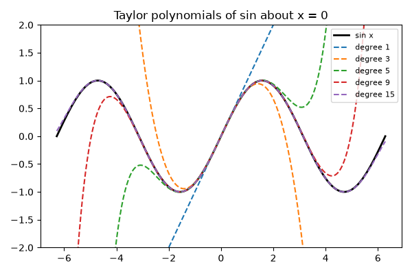
Taylor’s theorem expands a function in powers of \(x - x_0\) built from its derivatives at one point, with a Lagrange remainder \(|R_n(x)| \le M|x-x_0|^{n+1}/(n+1)!\). This example draws the Taylor (Maclaurin, \(x_0 = 0\)) polynomials of \(\sin\) closing in on the function, checks the true error against taylor_remainder_bound(), and shows what happens outside a series’ radius of convergence, where adding terms no longer helps.

import matplotlib.pyplot as plt
import numpy as np

from mathematicskit.calculus.systems.taylor_series import estimate_radius_of_convergence, evaluate_series, maclaurin_coefficients, taylor_remainder_bound
from mathematicskit.calculus.utils.series_utils import truncation_error

Taylor polynomials of sin approach the function

sin_coeffs = maclaurin_coefficients("sin", order=15)
grid = np.linspace(-2 * np.pi, 2 * np.pi, 400)
fig, ax = plt.subplots(figsize=(6, 4))
ax.plot(grid, np.sin(grid), "k", lw=2, label="sin x")
for degree in (1, 3, 5, 9, 15):
    ax.plot(grid, evaluate_series(sin_coeffs[: degree + 1], grid), "--", label=f"degree {degree}")
ax.set_ylim(-2, 2)
ax.set_title("Taylor polynomials of sin about x = 0")
ax.legend(fontsize=8)
fig.tight_layout()

The Lagrange remainder bounds the true error

Every derivative of \(\sin\) is bounded by \(M = 1\), so Taylor’s theorem guarantees \(|R_n(x)| \le |x|^{n+1}/(n+1)!\).

x = 1.5
for degree in (1, 3, 5, 7, 9):
    actual = abs(np.sin(x) - evaluate_series(sin_coeffs[: degree + 1], x))
    bound = taylor_remainder_bound(1.0, degree, x)
    print(f"degree {degree}: |error|={actual:.3e} <= bound {bound:.3e}: {actual <= bound}")

degree 1: |error|=5.025e-01 <= bound 1.125e+00: True
degree 3: |error|=5.999e-02 <= bound 2.109e-01: True
degree 5: |error|=3.286e-03 <= bound 1.582e-02: True
degree 7: |error|=1.038e-04 <= bound 6.356e-04: True
degree 9: |error|=2.136e-06 <= bound 1.589e-05: True

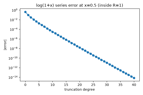
Convergence inside the radius: log(1+x) at x=0.5 (R=1)

coeffs = maclaurin_coefficients("log1p", order=40)
errors = truncation_error(np.log1p, coeffs, 0.5)

fig, ax = plt.subplots(figsize=(6, 4))
ax.semilogy(np.arange(len(errors)), np.maximum(errors, 1e-16), "o-")
ax.set_xlabel("truncation degree")
ax.set_ylabel("|error|")
ax.set_title("log(1+x) series error at x=0.5 (inside R=1)")
fig.tight_layout()

Failure to converge outside the radius: log(1+x) at x=1.5 (R=1)

errors_outside = truncation_error(np.log1p, coeffs, 1.5)
print("error at degree 10 (x=1.5, outside R=1):", errors_outside[10])
print("error at degree 39 (x=1.5, outside R=1):", errors_outside[39])
print("(error should be growing, not shrinking, since |x| > R)")

error at degree 10 (x=1.5, outside R=1): 3.3193878300884414
error at degree 39 (x=1.5, outside R=1): 112239.75068164946
(error should be growing, not shrinking, since |x| > R)

Radius-of-convergence estimates for each series

for name in ("exp", "sin", "cos", "log1p", "geometric", "arctan"):
    c = maclaurin_coefficients(name, order=30)
    print(f"{name:>10s}: estimated R ~ {estimate_radius_of_convergence(c):.4f}")

print("value check exp(1) via series:", evaluate_series(maclaurin_coefficients("exp", 20), 1.0), "vs.", np.e)

plt.show()

       exp: estimated R ~ inf
       sin: estimated R ~ inf
       cos: estimated R ~ inf
     log1p: estimated R ~ 1.0345
 geometric: estimated R ~ 1.0000
    arctan: estimated R ~ 1.0364
value check exp(1) via series: 2.718281828459045 vs. 2.718281828459045