De Casteljau’s algorithm and Bézier curves

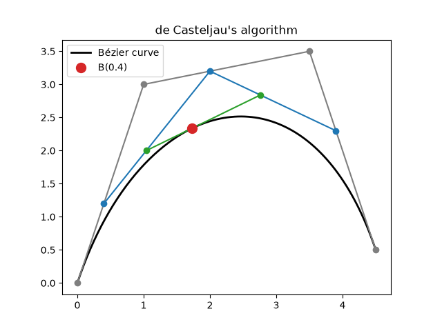
Draws a cubic Bézier curve and the construction lines of de Casteljau’s algorithm at t = 0.4: interpolate between neighbouring control points, then between the new points, until one point, the curve point, is left.

import matplotlib.pyplot as plt
import numpy as np

from mathematicskit.geometry import bezier_curve, de_casteljau

The construction at t = 0.4

control = np.array([[0.0, 0.0], [1.0, 3.0], [3.5, 3.5], [4.5, 0.5]])
curve = bezier_curve(control, np.linspace(0, 1, 200))
levels = de_casteljau(control, 0.4)

fig, ax = plt.subplots()
ax.plot(*curve.T, "k", lw=2, label="Bézier curve")
for level, color in zip(levels, ("tab:gray", "tab:blue", "tab:green", "tab:red")):
    ax.plot(*level.T, "o-", color=color, ms=6)
ax.plot(*levels[-1][0], "o", color="tab:red", ms=10, label="B(0.4)")
ax.set_aspect("equal")
ax.legend()
ax.set_title("de Casteljau's algorithm")

Text(0.5, 1.0, "de Casteljau's algorithm")

The curve stays inside the convex hull of its control points

print(f"curve x range [{curve[:, 0].min():.3f}, {curve[:, 0].max():.3f}], control x range [0, 4.5]")
print(f"curve starts at {curve[0]} and ends at {curve[-1]}: the first and last control points")

curve x range [0.000, 4.500], control x range [0, 4.5]
curve starts at [0. 0.] and ends at [4.5 0.5]: the first and last control points