Erdős and Rényi: the birth of the giant component

Samples random graphs G(n, c/n) and measures the largest connected component. Below the threshold c = 1 all components are tiny; above it a single giant component holds a fixed fraction s of the vertices, the root of s = 1 - exp(-c s).

import matplotlib.pyplot as plt
import numpy as np
from scipy.optimize import brentq

from mathematicskit.graph_theory import giant_component_fraction, random_graph

Simulation against the theoretical curve

n = 1500
cs = np.linspace(0.2, 3.0, 15)
measured = [np.mean([giant_component_fraction(random_graph(n, c / n, seed=s)) for s in range(3)]) for c in cs]
theory = [0.0 if c <= 1 else brentq(lambda s, c=c: s - 1 + np.exp(-c * s), 1e-9, 1.0) for c in cs]
for c, m, t in zip(cs[::3], measured[::3], theory[::3]):
    print(f"c = {c:.1f}: largest component {m:.3f} of the vertices (theory {t:.3f})")

fig, ax = plt.subplots()
ax.plot(cs, measured, "o", label=f"simulation, n = {n}")
ax.plot(cs, theory, "-", label=r"$s = 1 - e^{-cs}$")
ax.axvline(1.0, color="0.6", ls=":")
ax.set_xlabel("average degree c")
ax.set_ylabel("fraction in the largest component")
ax.legend()

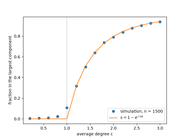
c = 0.2: largest component 0.004 of the vertices (theory 0.000)
c = 0.8: largest component 0.023 of the vertices (theory 0.000)
c = 1.4: largest component 0.503 of the vertices (theory 0.511)
c = 2.0: largest component 0.792 of the vertices (theory 0.797)
c = 2.6: largest component 0.904 of the vertices (theory 0.905)

<matplotlib.legend.Legend object at 0x1192f86e0>