Kruskal’s vs. Prim’s minimum spanning tree

Both algorithms find the same minimum spanning tree (same total weight) via very different strategies: Kruskal grows a forest by globally cheapest edge, Prim grows a single tree by locally cheapest edge.

from mathematicskit.graph_theory import Graph, kruskal_mst, prim_mst
from mathematicskit.graph_theory.visualizers.plots import plot_graph

Build a weighted graph

g = Graph(5)
g.add_edge(0, 1, 2.0)
g.add_edge(0, 3, 6.0)
g.add_edge(1, 2, 3.0)
g.add_edge(1, 3, 8.0)
g.add_edge(1, 4, 5.0)
g.add_edge(2, 4, 7.0)
g.add_edge(3, 4, 9.0)

Run both algorithms

kruskal_result = kruskal_mst(g)
prim_result = prim_mst(g)
print(f"Kruskal: {kruskal_result.edges}, total weight = {kruskal_result.total_weight}")
print(f"Prim:    {prim_result.edges}, total weight = {prim_result.total_weight}")

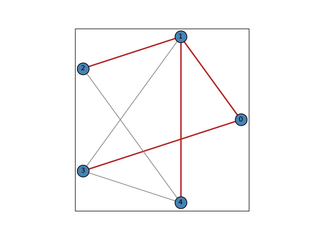
Kruskal: [(0, 1, 2.0), (0, 3, 6.0), (1, 2, 3.0), (1, 4, 5.0)], total weight = 16.0
Prim:    [(0, 1, 2.0), (1, 2, 3.0), (1, 4, 5.0), (0, 3, 6.0)], total weight = 16.0

Visualize the MST highlighted over the full graph

plot_graph(g, highlight_edges=[(u, v) for u, v, _w in kruskal_result.edges])

<Axes: >