Rate-distortion theory (1959)

If some error is allowed, fewer bits are needed. Shannon’s rate-distortion function \(R(D)\) is the fewest bits per symbol that reproduce a source within average distortion \(D\): for a fair coin with Hamming distortion \(R(D) = 1 - h(D)\), and for a Gaussian with squared error \(R(D) = \tfrac12\log_2(\sigma^2/D)\), 6.02 dB of quality per bit.

import matplotlib.pyplot as plt
import numpy as np

from mathematicskit.information_theory import rate_distortion_binary, rate_distortion_gaussian

fig, (ax1, ax2) = plt.subplots(1, 2, figsize=(11, 4))
D = np.linspace(0, 0.5, 300)
for p in (0.5, 0.25, 0.1):
    ax1.plot(D, rate_distortion_binary(D, p), label=f"Bernoulli({p})")
ax1.set_xlabel("allowed bit-error rate D")
ax1.set_ylabel("R(D) (bits per symbol)")
ax1.legend()

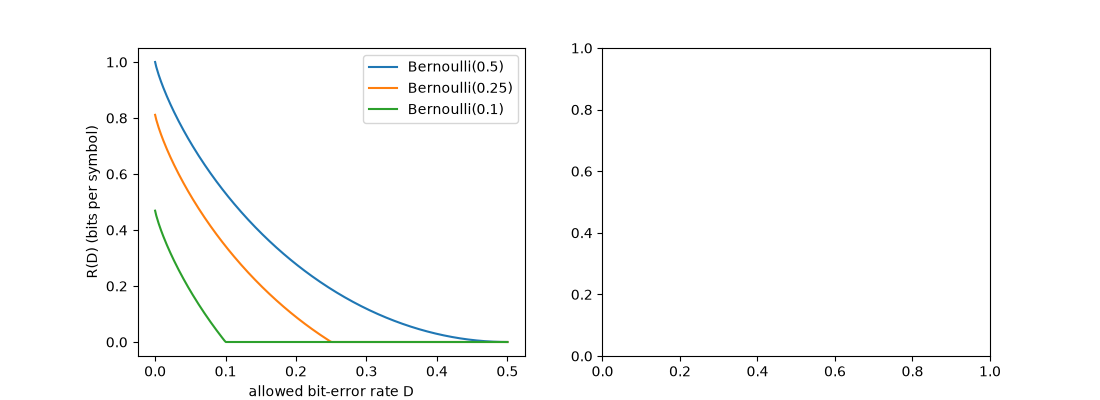
<matplotlib.legend.Legend object at 0x113530050>

Uniform scalar quantizers against the Gaussian bound

rng = np.random.default_rng(0)
x = rng.standard_normal(200_000)
bits, mse = [], []
for b in range(1, 7):
    levels = 2**b
    edges = np.linspace(-4, 4, levels + 1)
    centers = (edges[:-1] + edges[1:]) / 2
    xq = centers[np.clip(np.digitize(x, edges) - 1, 0, levels - 1)]
    bits.append(b)
    mse.append(np.mean((x - xq) ** 2))
Dg = np.logspace(-4, 0, 200)
ax2.plot(rate_distortion_gaussian(Dg), 10 * np.log10(Dg), label="R(D) bound")
ax2.plot(bits, 10 * np.log10(mse), "o-", label="uniform quantizer")
ax2.set_xlabel("bits per sample")
ax2.set_ylabel("distortion (dB)")
ax2.set_title("Gaussian source, squared error")
ax2.legend()

<matplotlib.legend.Legend object at 0x11359a7b0>