The Cayley-Hamilton theorem

Every square matrix satisfies its own characteristic equation: if p(l) = det(l I - A), then p(A) = 0. A consequence is that A^{-1} (and every higher power of A) is a polynomial in A of degree below n.

import matplotlib.pyplot as plt
import numpy as np

from mathematicskit.linalg import characteristic_polynomial, matrix_polynomial
from mathematicskit.linalg.visualizers.plots import plot_matrix_heatmap

Cayley’s 2x2 case

For a 2x2 matrix, p(l) = l^2 - tr(A) l + det(A).

A = np.array([[1.0, 2.0], [3.0, 4.0]])
p = characteristic_polynomial(A)
print("p(l) coefficients:", np.round(p, 10))
print("p(A) =\n", np.round(matrix_polynomial(p, A), 12))

p(l) coefficients: [ 1. -5. -2.]
p(A) =
 [[0. 0.]
 [0. 0.]]

A 5x5 random matrix, and the inverse as a polynomial

From p(A) = 0: A^{-1} = -(A^{n-1} + c_1 A^{n-2} + … + c_{n-1} I) / c_n.

rng = np.random.default_rng(1)
B = rng.normal(size=(5, 5))
c = characteristic_polynomial(B)
residual = matrix_polynomial(c, B)
print(f"||p(B)||_F = {np.linalg.norm(residual):.2e}")
B_inv = -matrix_polynomial(c[:-1], B) / c[-1]
print(f"||B^-1 (Cayley-Hamilton) - inv(B)||_F = {np.linalg.norm(B_inv - np.linalg.inv(B)):.2e}")

fig, axes = plt.subplots(1, 2, figsize=(8, 3.5))
plot_matrix_heatmap(B @ B, ax=axes[0], title="B^2")
plot_matrix_heatmap(residual, ax=axes[1], title="p(B) (rounding error only)")
fig.tight_layout()

plt.show()

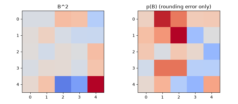
||p(B)||_F = 2.00e-14
||B^-1 (Cayley-Hamilton) - inv(B)||_F = 1.72e-14