Lanczos: a few eigenvalues of a very large matrix

The 1-D discrete Laplacian tridiag(-1, 2, -1) of size n has eigenvalues 2 - 2 cos(j pi / (n + 1)). Lanczos iteration (through ARPACK) finds a handful of them using only matrix-vector products. In shift-invert mode it handles a sparse n = 100 000 instance, where a dense eigensolver would need 80 GB just to store the matrix.

import matplotlib.pyplot as plt
import numpy as np
import scipy.sparse as sp

from mathematicskit.linalg import lanczos_eigsh


def laplacian_1d(n):
    return sp.diags([-np.ones(n - 1), 2 * np.ones(n), -np.ones(n - 1)], [-1, 0, 1], format="csc")


def exact(j, n):
    return 2.0 - 2.0 * np.cos(j * np.pi / (n + 1))

Largest eigenvalues by plain Lanczos

n = 2000
result = lanczos_eigsh(laplacian_1d(n), k=4, which="LA")
for lam, ex in zip(result.eigenvalues, exact(np.arange(n - 3, n + 1), n)):
    print(f"Lanczos {lam:.14f}   exact {ex:.14f}   |diff| {abs(lam - ex):.1e}")

Lanczos 3.99996056116101   exact 3.99996056116084   |diff| 1.6e-13
Lanczos 3.99997781562106   exact 3.99997781562108   |diff| 1.8e-14
Lanczos 3.99999014026616   exact 3.99999014026591   |diff| 2.6e-13
Lanczos 3.99999753506495   exact 3.99999753506496   |diff| 4.0e-15

Smallest eigenvalues of n = 100 000, by shift-invert Lanczos

n = 100_000
result = lanczos_eigsh(laplacian_1d(n), k=4, sigma=0.0, which="LM")
for lam, ex in zip(result.eigenvalues, exact(np.arange(1, 5), n)):
    print(f"Lanczos {lam:.6e}   exact {ex:.6e}   rel. error {abs(lam - ex) / ex:.1e}")

fig, ax = plt.subplots(figsize=(6, 4))
for k in range(3):
    v = result.eigenvectors[:, k]
    ax.plot(np.sign(v[n // 10]) * v, label=f"lambda_{k + 1} = {result.eigenvalues[k]:.3e}")
ax.set_xlabel("index")
ax.set_title("Lowest Laplacian eigenvectors: sine modes")
ax.legend()
fig.tight_layout()

plt.show()

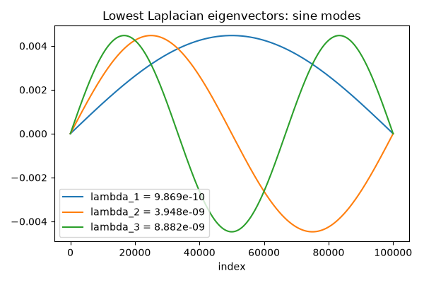
Lanczos 9.869407e-10   exact 9.869408e-10   rel. error 5.1e-08
Lanczos 3.947763e-09   exact 3.947763e-09   rel. error 5.2e-09
Lanczos 8.882466e-09   exact 8.882466e-09   rel. error 1.5e-09
Lanczos 1.579105e-08   exact 1.579105e-08   rel. error 4.1e-09