Jacobi, Gauss-Seidel, and successive over-relaxation

The three classical stationary iterations on the 1-D Poisson matrix tridiag(-1, 2, -1). Gauss-Seidel contracts the error about twice as fast per sweep as Jacobi, and SOR at Young’s optimal relaxation factor is faster by an order of magnitude.

import matplotlib.pyplot as plt
import numpy as np

from mathematicskit.linalg import SOR, GaussSeidel, JacobiIteration, jacobi_spectral_radius, optimal_sor_omega
from mathematicskit.linalg.visualizers.plots import plot_residual_history

Spectral radii predicted by Young’s theory

n = 40
A = 2.0 * np.eye(n) - np.eye(n, k=1) - np.eye(n, k=-1)
b = np.ones(n)
rho_j = jacobi_spectral_radius(A)
omega = optimal_sor_omega(A)
print(f"rho(Jacobi) = {rho_j:.6f}   (cos(pi/(n+1)) = {np.cos(np.pi / (n + 1)):.6f})")
print(f"rho(Gauss-Seidel) = rho(Jacobi)^2 = {rho_j**2:.6f}")
print(f"optimal omega = {omega:.6f}, rho(SOR) = omega - 1 = {omega - 1:.6f}")

rho(Jacobi) = 0.997066   (cos(pi/(n+1)) = 0.997066)
rho(Gauss-Seidel) = rho(Jacobi)^2 = 0.994140
optimal omega = 1.857788, rho(SOR) = omega - 1 = 0.857788

Convergence histories

results = [
    JacobiIteration(tol=1e-8, max_iter=20000).solve(A, b),
    GaussSeidel(tol=1e-8, max_iter=20000).solve(A, b),
    SOR(omega=omega, tol=1e-8, max_iter=20000).solve(A, b),
]
for r in results:
    print(f"{r.method:13s}: {r.iterations:5d} sweeps")

fig, ax = plt.subplots(figsize=(6, 4))
for r in results:
    plot_residual_history(r, ax=ax)
ax.legend()
fig.tight_layout()

plt.show()

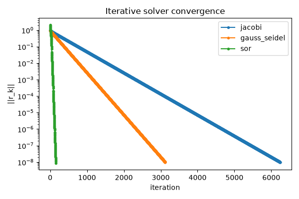
jacobi       :  6238 sweeps
gauss_seidel :  3120 sweeps
sor          :   152 sweeps