Turing’s condition number: how much a linear system amplifies error

kappa_2(A) = sigma_max / sigma_min bounds how much a relative perturbation of the data can grow in the solution of A x = b, whichever algorithm solves it: expect to lose about log10(kappa) digits. The same number explains why least squares through the normal equations A^T A x = A^T b is fragile – kappa(A^T A) = kappa(A)^2 – while QR works with kappa(A) itself.

import matplotlib.pyplot as plt
import numpy as np
from scipy.linalg import hilbert

from mathematicskit.linalg import condition_number_2norm, least_squares_normal_equations, least_squares_qr, lu_solve_system, svd_decompose

eps = np.finfo(float).eps

The condition number is a ratio of singular values

H = hilbert(6)
S = svd_decompose(H).S
print(f"sigma_max / sigma_min = {S.max() / S.min():.4e}")
print(f"condition_number_2norm = {condition_number_2norm(H):.4e}")

sigma_max / sigma_min = 1.4951e+07
condition_number_2norm = 1.4951e+07

Error amplification: the bound is attained

Take x along the top right singular vector and perturb b by a tiny relative amount along the worst direction (the left singular vector of sigma_min): the relative change in x is exactly kappa times larger.

res = svd_decompose(H)
x = res.Vt[np.argmax(res.S)]
b = H @ x
db = 1e-10 * np.linalg.norm(b) * res.U[:, np.argmin(res.S)]
dx = lu_solve_system(H, b + db) - x
amplification = (np.linalg.norm(dx) / np.linalg.norm(x)) / (np.linalg.norm(db) / np.linalg.norm(b))
print(f"relative error amplification = {amplification:.4e}  (kappa = {condition_number_2norm(H):.4e})")

relative error amplification = 1.4951e+07  (kappa = 1.4951e+07)

Digits lost on Hilbert matrices

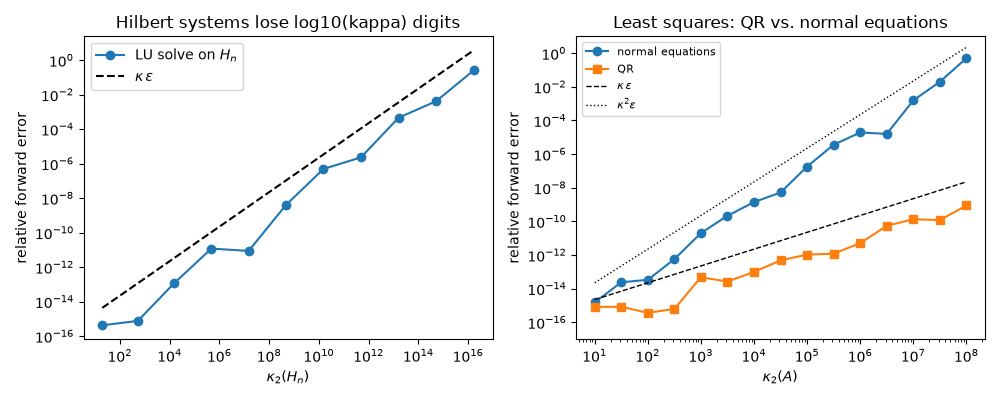
Solving H_n x = H_n 1 in double precision: the forward error tracks kappa(H_n) * eps.

ns = np.arange(2, 13)
kappas, errors = [], []
for n in ns:
    Hn = hilbert(n)
    xn = lu_solve_system(Hn, Hn @ np.ones(n))
    kappas.append(condition_number_2norm(Hn))
    errors.append(np.linalg.norm(xn - 1.0) / np.sqrt(n))
    print(f"n = {n:2d}: kappa = {kappas[-1]:.2e}, relative error = {errors[-1]:.2e}")

n =  2: kappa = 1.93e+01, relative error = 4.23e-16
n =  3: kappa = 5.24e+02, relative error = 7.61e-16
n =  4: kappa = 1.55e+04, relative error = 1.21e-13
n =  5: kappa = 4.77e+05, relative error = 1.18e-11
n =  6: kappa = 1.50e+07, relative error = 8.63e-12
n =  7: kappa = 4.75e+08, relative error = 4.01e-09
n =  8: kappa = 1.53e+10, relative error = 4.88e-07
n =  9: kappa = 4.93e+11, relative error = 2.31e-06
n = 10: kappa = 1.60e+13, relative error = 4.55e-04
n = 11: kappa = 5.22e+14, relative error = 4.16e-03
n = 12: kappa = 1.72e+16, relative error = 2.61e-01

Least squares: kappa for QR, kappa squared for the normal equations

Build 40x5 design matrices with prescribed condition number and compare the two solvers’ forward errors.

rng = np.random.default_rng(6)
U, _ = np.linalg.qr(rng.normal(size=(40, 5)))
V, _ = np.linalg.qr(rng.normal(size=(5, 5)))
x_true = np.array([1.0, -2.0, 0.5, 3.0, -1.5])
targets = np.logspace(1, 8, 15)
err_normal, err_qr = [], []
for kappa in targets:
    A = U @ np.diag(np.logspace(0, -np.log10(kappa), 5)) @ V.T
    b = A @ x_true
    for solver, store in ((least_squares_normal_equations, err_normal), (least_squares_qr, err_qr)):
        coef = solver(A, b).coefficients
        store.append(np.linalg.norm(coef - x_true) / np.linalg.norm(x_true))

A = U @ np.diag(np.logspace(0, -4, 5)) @ V.T
print(f"kappa(A) = {condition_number_2norm(A):.3e}, kappa(A^T A) = {condition_number_2norm(A.T @ A):.3e}")

fig, axes = plt.subplots(1, 2, figsize=(10, 4))
ax = axes[0]
ax.loglog(kappas, errors, "o-", label="LU solve on $H_n$")
ax.loglog(kappas, np.array(kappas) * eps, "k--", label=r"$\kappa\,\varepsilon$")
ax.set_xlabel(r"$\kappa_2(H_n)$")
ax.set_ylabel("relative forward error")
ax.set_title("Hilbert systems lose log10(kappa) digits")
ax.legend()

ax = axes[1]
ax.loglog(targets, err_normal, "o-", label="normal equations")
ax.loglog(targets, err_qr, "s-", label="QR")
ax.loglog(targets, targets * eps, "k--", lw=1, label=r"$\kappa\,\varepsilon$")
ax.loglog(targets, targets**2 * eps, "k:", lw=1, label=r"$\kappa^2\varepsilon$")
ax.set_ylim(1e-17, 10)
ax.set_xlabel(r"$\kappa_2(A)$")
ax.set_ylabel("relative forward error")
ax.set_title("Least squares: QR vs. normal equations")
ax.legend(fontsize=8)
fig.tight_layout()

plt.show()

kappa(A) = 1.000e+04, kappa(A^T A) = 1.000e+08