The Moore-Penrose pseudoinverse

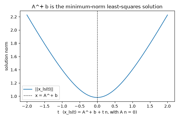
For a rectangular or rank-deficient A there is no inverse, but there is exactly one matrix A^+ satisfying Penrose’s four equations, and x = A^+ b is the shortest vector among all least-squares solutions.

import matplotlib.pyplot as plt
import numpy as np

from mathematicskit.linalg import penrose_residuals, pseudoinverse

A rank-deficient system

The third column is the sum of the first two, so A has rank 2 and the least-squares solutions form a line in R^3.

A = np.array([[1.0, 0.0, 1.0], [0.0, 1.0, 1.0], [1.0, 1.0, 2.0], [1.0, -1.0, 0.0]])
b = np.array([1.0, 2.0, 2.0, 0.0])
A_plus = pseudoinverse(A)
x_plus = A_plus @ b
print("rank(A) =", np.linalg.matrix_rank(A))
print("Penrose residuals:", np.array2string(penrose_residuals(A, A_plus), precision=1))
print("x = A^+ b =", np.round(x_plus, 6))

null = np.array([1.0, 1.0, -1.0]) / np.sqrt(3.0)  # A @ null = 0
ts = np.linspace(-2, 2, 201)
norms = [np.linalg.norm(x_plus + t * null) for t in ts]
residuals = [np.linalg.norm(A @ (x_plus + t * null) - b) for t in ts]
print(f"residual along the solution line is constant: {min(residuals):.6f} .. {max(residuals):.6f}")

fig, ax = plt.subplots(figsize=(6, 4))
ax.plot(ts, norms, label="||x_ls(t)||")
ax.axvline(0.0, color="k", ls="--", lw=0.8, label="x = A^+ b")
ax.set_xlabel("t   (x_ls(t) = A^+ b + t n, with A n = 0)")
ax.set_ylabel("solution norm")
ax.set_title("A^+ b is the minimum-norm least-squares solution")
ax.legend()
fig.tight_layout()

plt.show()

rank(A) = 2
Penrose residuals: [9.1e-16 2.0e-16 2.5e-16 1.8e-16]
x = A^+ b = [0.222222 0.555556 0.777778]
residual along the solution line is constant: 0.816497 .. 0.816497