The Lenstra-Lenstra-Lovász lattice reduction algorithm

A lattice has infinitely many bases, and a basis of long, nearly parallel vectors hides its structure. Lenstra, Lenstra and Lovász (1982) gave a polynomial-time algorithm that turns any basis into a reduced one, of short and nearly orthogonal vectors. They needed it to factor polynomials with rational coefficients; it has since become a universal tool, from breaking knapsack cryptosystems to discovering integer relations among real numbers.

import math

import matplotlib.pyplot as plt
import numpy as np

from mathematicskit.number_theory import integer_relation, lll_reduce

A bad basis and a good one for the same lattice

The vectors \((201, 37)\) and \((1648, 297)\) generate the same lattice as \((1, 32)\) and \((40, 1)\); the determinant, the area of the fundamental parallelogram, is the same 1279.

bad = [[201, 37], [1648, 297]]
good = lll_reduce(bad)
print(f"reduced basis {good.basis} after {good.swaps} swaps")
print(f"|det|: {abs(np.linalg.det(bad)):.0f} vs {abs(np.linalg.det(good.basis)):.0f}")

coefficients = np.array([(i, j) for i in range(-60, 61) for j in range(-60, 61)])
lattice_points = coefficients @ np.array(good.basis)
fig, (ax0, ax1, ax2) = plt.subplots(1, 3, figsize=(16, 5))
view = (np.abs(lattice_points) < 200).all(axis=1)
ax0.plot(*lattice_points[view].T, ".", color="0.6", ms=3)
for (vx, vy), color, label in zip(bad + good.basis, ["tab:red", "tab:red", "tab:blue", "tab:blue"], ["input basis", None, "LLL basis", None], strict=True):
    ax0.annotate("", (vx, vy), (0, 0), arrowprops={"arrowstyle": "-|>", "color": color, "lw": 2})
    if label:
        ax0.plot([], [], color=color, lw=2, label=label)
ax0.set_xlim(-200, 1700)
ax0.set_ylim(-200, 320)
ax0.set_title("Same lattice, two bases")
ax0.legend(loc="lower right")

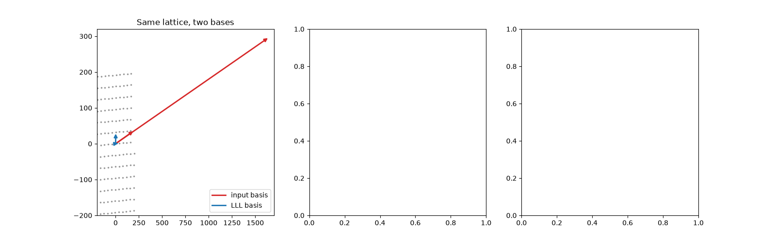
reduced basis [[1, 32], [40, 1]] after 2 swaps
|det|: 1279 vs 1279

<matplotlib.legend.Legend object at 0x113363b60>

Gram-Schmidt profile of a random lattice

LLL’s Lovász condition stops the Gram-Schmidt lengths \(\|b_i^*\|\) from falling faster than a fixed ratio; the first vector comes out short, within \(2^{(n-1)/2}\) of the shortest lattice vector.

rng = np.random.default_rng(1982)
n = 12
basis = rng.integers(-100, 101, size=(n, n)).tolist()
before = np.abs(np.diag(np.linalg.qr(np.array(basis, dtype=float).T)[1]))  # |R_ii| = ||b_i*||
reduced = lll_reduce(basis)
after = np.sqrt(reduced.gram_schmidt_norms)
shortest_input = min(np.linalg.norm(b) for b in basis)
print(f"{n}-dimensional lattice: shortest input vector {shortest_input:.0f}, first LLL vector {np.linalg.norm(reduced.basis[0]):.0f} ({reduced.swaps} swaps)")
ax1.semilogy(np.arange(1, n + 1), [np.linalg.norm(b) for b in basis], "o--", color="tab:red", label=r"$\|b_i\|$, input")
ax1.semilogy(np.arange(1, n + 1), before, "o-", color="tab:red", alpha=0.5, label=r"$\|b_i^*\|$, input")
ax1.semilogy(np.arange(1, n + 1), [np.linalg.norm(b) for b in reduced.basis], "s--", color="tab:blue", label=r"$\|b_i\|$, LLL")
ax1.semilogy(np.arange(1, n + 1), after, "s-", color="tab:blue", alpha=0.5, label=r"$\|b_i^*\|$, LLL")
ax1.set_xlabel("i")
ax1.set_title("Reduction flattens the Gram-Schmidt profile")
ax1.legend(fontsize=8)

12-dimensional lattice: shortest input vector 149, first LLL vector 102 (44 swaps)

<matplotlib.legend.Legend object at 0x112f93b60>

Recovering minimal polynomials from decimals

If \(\alpha\) is algebraic of degree \(d\), there are small integers with \(\sum_k a_k \alpha^k = 0\). Scaling the decimals by \(C\) and reducing the lattice of \([\,I \mid C\alpha^k\,]\) finds them.

numbers = {
    "sqrt(2) + sqrt(3)": (math.sqrt(2) + math.sqrt(3), 4),
    "2^(1/3) + 1": (2 ** (1 / 3) + 1, 3),
    "cos(2 pi / 7)": (math.cos(2 * math.pi / 7), 3),
    "golden ratio": ((1 + math.sqrt(5)) / 2, 2),
}


def polynomial_text(coefficients):
    """Format a_0 + a_1 x + ... highest degree first, e.g. "x^4 - 10x^2 + 1"."""
    text = ""
    for k in range(len(coefficients) - 1, -1, -1):
        a = coefficients[k]
        if a:
            monomial = "" if k == 0 else ("x" if k == 1 else f"x^{k}")
            magnitude = "" if abs(a) == 1 and k else str(abs(a))
            text += (" - " if a < 0 else " + ") + magnitude + monomial
    return text[3:]


for name, (alpha, degree) in numbers.items():
    relation = integer_relation([alpha**k for k in range(degree + 1)], scale=1e10)
    relation = relation if relation[-1] > 0 else [-a for a in relation]  # positive leading coefficient
    residual = sum(a * alpha**k for k, a in enumerate(relation))
    print(f"{name:18s} {polynomial_text(relation):24s} residual {residual:.1e}")

# Too little precision gives a spurious relation: the scale must exceed
# roughly the product of the coefficients' sizes.
scales = np.logspace(2, 12, 21)
alpha = math.sqrt(2) + math.sqrt(3)
found = [integer_relation([alpha**k for k in range(5)], scale=s) == [1, 0, -10, 0, 1] for s in scales]
ax2.semilogx(scales, found, "o-")
ax2.set_yticks([0, 1], ["spurious", r"$x^4 - 10x^2 + 1$"])
ax2.set_xlabel("scale C (digits of precision used)")
ax2.set_title(r"Minimal polynomial of $\sqrt{2} + \sqrt{3}$")
fig.tight_layout()

plt.show()

sqrt(2) + sqrt(3)  x^4 - 10x^2 + 1          residual 1.4e-14
2^(1/3) + 1        x^3 - 3x^2 + 3x - 3      residual 8.9e-16
cos(2 pi / 7)      8x^3 + 4x^2 - 4x - 1     residual 6.7e-16
golden ratio       x^2 - x - 1              residual 0.0e+00