Euler’s method: first-order convergence

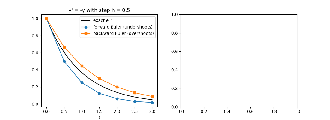
Euler (1768) replaced the curve by its tangent line over a short step \(h\): \(y_{n+1} = y_n + h f(t_n, y_n)\). Evaluating the slope at the end of the step instead gives the implicit (backward) variant \(y_{n+1} = y_n + h f(t_{n+1}, y_{n+1})\). Both have a local error of \(O(h^2)\), which adds up to a global error of \(O(h)\): halving the step halves the error.

import matplotlib.pyplot as plt
import numpy as np

from mathematicskit.integrators import euler_integrate, implicit_euler_integrate, njit


@njit
def decay(state, t, params):
    return -state


def forward_euler(y0, h, n_steps):
    return euler_integrate(decay, np.array([y0]), 0.0, h, n_steps, np.zeros(1))[1][:, 0]

Tangent-line steps

h, n = 0.5, 6
ts = h * np.arange(n + 1)
_, ys_back = implicit_euler_integrate(decay, np.array([1.0]), 0.0, h, n, np.zeros(1))
t_fine = np.linspace(0.0, n * h, 200)

fig, (ax0, ax1) = plt.subplots(1, 2, figsize=(11, 4))
ax0.plot(t_fine, np.exp(-t_fine), "k", label=r"exact $e^{-t}$")
ax0.plot(ts, forward_euler(1.0, h, n), "o-", label="forward Euler (undershoots)")
ax0.plot(ts, ys_back[:, 0], "s-", label="backward Euler (overshoots)")
ax0.set_xlabel("t")
ax0.set_title(f"y' = -y with step h = {h}")
ax0.legend()

<matplotlib.legend.Legend object at 0x7fd7c2f39e80>

Global error is proportional to h

hs = 1.0 / 2 ** np.arange(3, 11)
err_fwd = [abs(forward_euler(1.0, h, round(1 / h))[-1] - np.exp(-1)) for h in hs]
err_back = [abs(implicit_euler_integrate(decay, np.array([1.0]), 0.0, h, round(1 / h), np.zeros(1))[1][-1, 0] - np.exp(-1)) for h in hs]
ax1.loglog(hs, err_fwd, "o-", label="forward Euler")
ax1.loglog(hs, err_back, "s-", label="backward Euler")
ax1.loglog(hs, 0.2 * hs, "k--", label=r"slope 1: $O(h)$")
ax1.set_xlabel("h")
ax1.set_ylabel("|error| at t = 1")
ax1.set_title("First-order convergence")
ax1.legend()
fig.tight_layout()

print(f"error ratio for halved h: forward {err_fwd[-2] / err_fwd[-1]:.3f}, backward {err_back[-2] / err_back[-1]:.3f}")

plt.show()

error ratio for halved h: forward 2.001, backward 1.999