Dormand-Prince: embedded pairs and adaptive step size

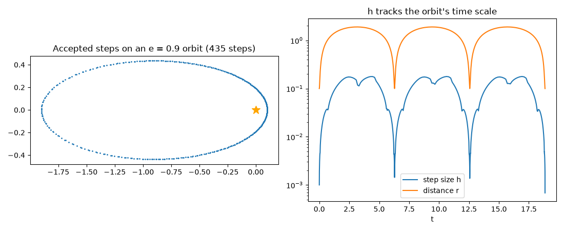
An embedded Runge-Kutta pair computes a 5th- and a 4th-order solution from the same seven stages. Their difference estimates the local error at almost no extra cost. Dormand and Prince (1980) tuned the pair so that the 5th-order result, the one actually kept, has a very small error constant. A controller then shrinks \(h\) where the error estimate is large and grows it where it is small. On a highly eccentric Kepler orbit the step collapses at each close pass (perihelion) and stretches out far from the Sun (aphelion).

import matplotlib.pyplot as plt
import numpy as np

from mathematicskit.integrators import dopri5_integrate, njit


@njit
def kepler(state, t, params):
    r3 = (state[0] ** 2 + state[1] ** 2) ** 1.5
    return np.array([state[2], state[3], -state[0] / r3, -state[1] / r3])


e = 0.9
state0 = np.array([1.0 - e, 0.0, 0.0, np.sqrt((1 + e) / (1 - e))])  # perihelion, semi-major axis 1
period = 2 * np.pi

Steps crowd around perihelion

ts, ys = dopri5_integrate(kepler, state0, 0.0, 3 * period, 1e-3, np.zeros(1), rtol=1e-8, atol=1e-10)
r = np.hypot(ys[:, 0], ys[:, 1])

fig, (ax0, ax1) = plt.subplots(1, 2, figsize=(11, 4.5))
ax0.plot(ys[:, 0], ys[:, 1], ".", ms=2)
ax0.plot(0, 0, "*", color="orange", ms=12)
ax0.set_aspect("equal")
ax0.set_title(f"Accepted steps on an e = {e} orbit ({len(ts) - 1} steps)")

ax1.semilogy(ts[1:], np.diff(ts), label="step size h")
ax1.semilogy(ts, r, label="distance r")
ax1.set_xlabel("t")
ax1.set_title("h tracks the orbit's time scale")
ax1.legend()
fig.tight_layout()

Tolerance sets the cost

for rtol in (1e-4, 1e-6, 1e-8, 1e-10):
    ts_, ys_ = dopri5_integrate(kepler, state0, 0.0, period, 1e-3, np.zeros(1), rtol=rtol, atol=rtol * 1e-2)
    print(f"rtol={rtol:.0e}: {len(ts_) - 1:5d} steps, error after one period = {np.linalg.norm(ys_[-1] - state0):.2e}")

plt.show()

rtol=1e-04:    28 steps, error after one period = 1.41e+00
rtol=1e-06:    61 steps, error after one period = 1.97e-02
rtol=1e-08:   145 steps, error after one period = 1.22e-04
rtol=1e-10:   364 steps, error after one period = 7.02e-07