Stormer-Verlet: bounded energy error over long times

Stormer (1907) computed charged-particle orbits in the Earth’s magnetic field with the scheme later rediscovered by Verlet (1967) for molecular dynamics. For \(\ddot q = F(q)\):

\[v_{n+1/2} = v_n + \tfrac{h}{2}F(q_n),\quad q_{n+1} = q_n + h\,v_{n+1/2},\quad v_{n+1} = v_{n+1/2} + \tfrac{h}{2}F(q_{n+1}).\]

It is only second order, but it is symplectic: it exactly conserves a slightly perturbed energy. So its energy error stays bounded over arbitrarily long runs. RK4 is more accurate per step, but its energy error drifts steadily.

import matplotlib.pyplot as plt
import numpy as np

from mathematicskit.integrators import leapfrog_integrate, njit, rk4_integrate


@njit
def pendulum_force(q, t, params):
    return -np.sin(q)


@njit
def pendulum_rhs(state, t, params):
    return np.array([state[1], -np.sin(state[0])])


def energy(q, v):
    return 0.5 * v**2 - np.cos(q)

A pendulum released at 2.5 rad, integrated for about 1000 swings

h, n = 0.25, 30_000
q0, v0 = 2.5, 0.0
ts, qs, vs = leapfrog_integrate(pendulum_force, np.array([q0]), np.array([v0]), 0.0, h, n, np.zeros(1))
_, ys = rk4_integrate(pendulum_rhs, np.array([q0, v0]), 0.0, h, n, np.zeros(1))
e0 = energy(q0, v0)

fig, ax = plt.subplots(figsize=(8, 4.5))
ax.plot(ts, energy(ys[:, 0], ys[:, 1]) - e0, lw=0.8, label="RK4 (4th order)")
ax.plot(ts, energy(qs[:, 0], vs[:, 0]) - e0, lw=0.8, label="Stormer-Verlet (2nd order, symplectic)")
ax.set_xlabel("t")
ax.set_ylabel("E(t) - E(0)")
ax.set_title(f"Pendulum energy error, h = {h}")
ax.legend()
fig.tight_layout()

print(f"max |energy error|: Verlet {np.max(np.abs(energy(qs[:, 0], vs[:, 0]) - e0)):.2e}, RK4 {np.max(np.abs(energy(ys[:, 0], ys[:, 1]) - e0)):.2e}")

plt.show()

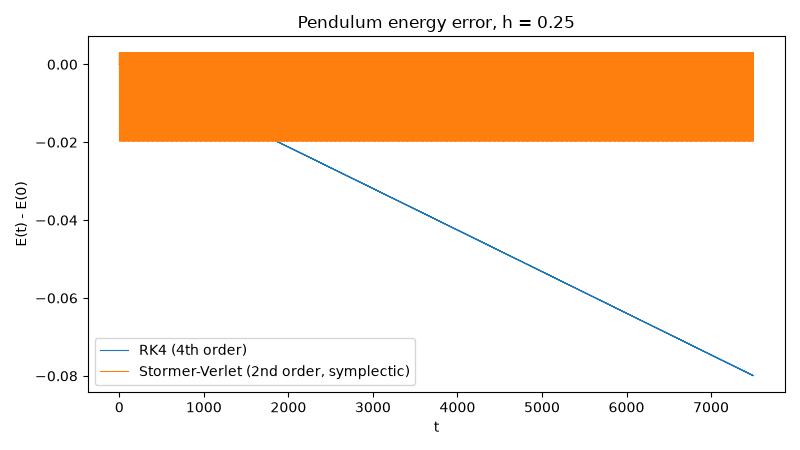
max |energy error|: Verlet 1.98e-02, RK4 8.00e-02