The Van der Pol limit cycle

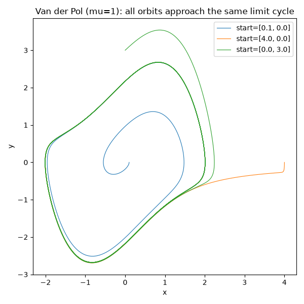
Trajectories starting both inside and outside the eventual limit cycle converge onto the same closed orbit – the defining property that distinguishes a limit cycle from a linear center (whose orbit amplitude is set entirely by the initial condition).

import matplotlib.pyplot as plt

from mathematicskit.ode_dynamics.systems.limit_cycles import VanDerPolOscillator, estimate_limit_cycle_amplitude
from mathematicskit.ode_dynamics.visualizers.plots import plot_phase_portrait

Trajectories from very different initial conditions converge

fig, ax = plt.subplots(figsize=(6, 6))
for state0 in ([0.1, 0.0], [4.0, 0.0], [0.0, 3.0]):
    system = VanDerPolOscillator(state0, mu=1.0)
    traj = system.integrate((0.0, 30.0), dt=1e-3, method="rk4")
    plot_phase_portrait(traj, ax=ax, lw=0.8, label=f"start={state0}")
ax.legend()
ax.set_title("Van der Pol (mu=1): all orbits approach the same limit cycle")
fig.tight_layout()

Amplitude is independent of mu’s transient details

for mu in (0.5, 1.0, 2.0, 5.0):
    amp = estimate_limit_cycle_amplitude(mu=mu, t_transient=150.0, t_observe=40.0)
    print(f"mu={mu}: limit-cycle amplitude ~ {amp:.4f}")

plt.show()

mu=0.5: limit-cycle amplitude ~ 2.0025
mu=1.0: limit-cycle amplitude ~ 2.0086
mu=2.0: limit-cycle amplitude ~ 2.0199
mu=5.0: limit-cycle amplitude ~ 2.0215