The Brusselator’s Hopf bifurcation

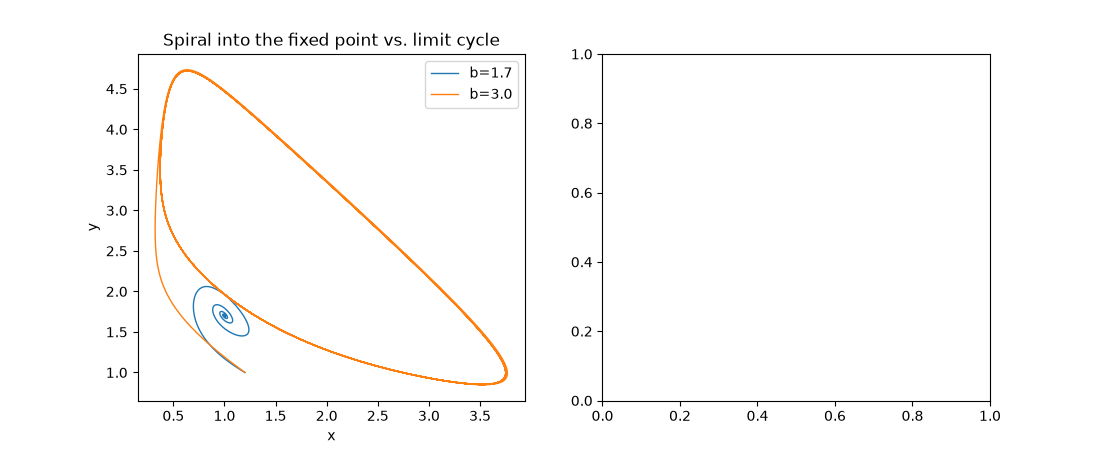
The Brusselator’s fixed point \((a, b/a)\) is stable until \(b\) crosses \(b_c = 1 + a^2\), where the trace of its Jacobian changes sign and a limit cycle is born: the model chemical reaction starts to oscillate.

import matplotlib.pyplot as plt
import numpy as np

from mathematicskit.ode_dynamics.systems.chemical_oscillators import Brusselator, brusselator_hopf_threshold

a = 1.0
b_c = brusselator_hopf_threshold(a)
print(f"Hopf threshold b_c = 1 + a^2 = {b_c}")

Hopf threshold b_c = 1 + a^2 = 2.0

Below and above the threshold

fig, axes = plt.subplots(1, 2, figsize=(11, 4.5))
for b in (1.7, 3.0):
    traj = Brusselator([1.2, 1.0], a=a, b=b).integrate((0.0, 60.0), dt=1e-2, method="rk4")
    axes[0].plot(traj.y[:, 0], traj.y[:, 1], lw=1, label=f"b={b}")
axes[0].set_xlabel("x")
axes[0].set_ylabel("y")
axes[0].set_title("Spiral into the fixed point vs. limit cycle")
axes[0].legend()

<matplotlib.legend.Legend object at 0x11aeeb380>

Oscillation amplitude across the bifurcation

bs = np.linspace(1.5, 3.5, 21)
amps = []
for b in bs:
    traj = Brusselator([1.2, 1.0], a=a, b=b).integrate((0.0, 300.0), dt=1e-2, method="rk4")
    amps.append(np.ptp(traj.y[-5000:, 0]))
axes[1].plot(bs, amps, "o-")
axes[1].axvline(b_c, color="gray", ls="--", label="b_c = 1 + a^2")
axes[1].set_xlabel("b")
axes[1].set_ylabel("peak-to-peak x")
axes[1].set_title("Oscillations switch on at b_c")
axes[1].legend()
fig.tight_layout()

plt.show()