Poincaré’s qualitative method: the pendulum’s phase portrait

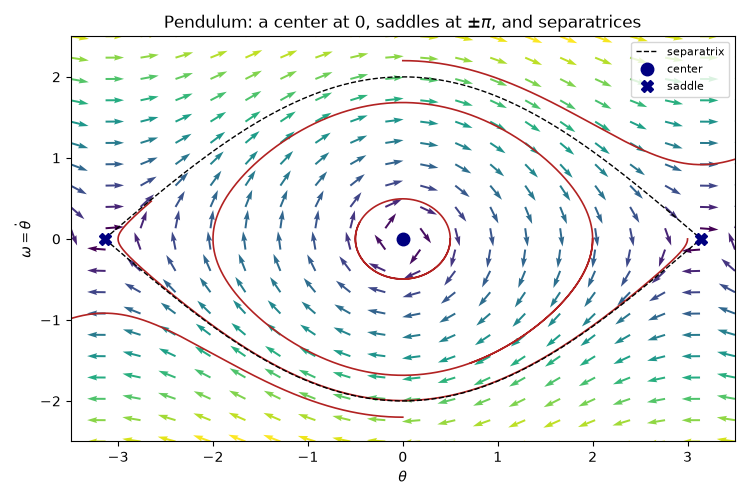
The nonlinear pendulum \(\ddot\theta = -\sin\theta\) has no elementary closed-form solution, but Poincaré’s qualitative approach does not need one. Locate the fixed points, classify each from its linearization, and sketch the vector field: the global picture of librating orbits around the centers, rotating orbits above and below, and separatrices joining the saddles follows without solving anything. Integrated trajectories are overlaid only to confirm the prediction.

import matplotlib.pyplot as plt
import numpy as np

from mathematicskit.ode_dynamics.systems.phase_portrait import Nonlinear2D, vector_field_grid
from mathematicskit.ode_dynamics.systems.stability import classify_fixed_point_2d, numerical_jacobian
from mathematicskit.ode_dynamics.visualizers.plots import plot_phase_portrait, plot_vector_field


def pendulum(theta, omega):
    return omega, -np.sin(theta)

Step 1: classify the fixed points

The fixed points are \((k\pi, 0)\). Linearizing shows the hanging positions are centers and the inverted positions are saddles.

fixed_points = {}
for theta_star in (-np.pi, 0.0, np.pi):
    p = np.array([theta_star, 0.0])
    J = numerical_jacobian(lambda s: np.array(pendulum(s[0], s[1])), p)
    result = classify_fixed_point_2d(J, location=p)
    fixed_points[theta_star] = result.classification
    print(f"theta* = {theta_star:+.4f}: eigenvalues={np.round(result.eigenvalues, 3)} -> {result.classification}")

theta* = -3.1416: eigenvalues=[ 1.+0.j -1.+0.j] -> saddle
theta* = +0.0000: eigenvalues=[0.+1.j 0.-1.j] -> center
theta* = +3.1416: eigenvalues=[ 1.+0.j -1.+0.j] -> saddle

Step 2: vector field, then trajectories as a check

The separatrix through the saddles has energy \(\tfrac12\omega^2 - \cos\theta = 1\), i.e. \(\omega = \pm 2\cos(\theta/2)\).

X, Y, U, V = vector_field_grid(pendulum, (-3.5, 3.5), (-2.5, 2.5), n=20)

fig, ax = plt.subplots(figsize=(7.5, 5))
plot_vector_field(X, Y, U, V, ax=ax)

trajectories = []
for theta0, omega0 in [(0.5, 0.0), (2.0, 0.0), (3.0, 0.0), (0.0, 2.2), (0.0, -2.2)]:
    system = Nonlinear2D([theta0, omega0], f=pendulum)
    trajectories.append(system.integrate((0.0, 10.0), dt=1e-3, method="rk4"))
plot_phase_portrait(trajectories, ax=ax, color="firebrick", lw=1.2)

theta = np.linspace(-np.pi, np.pi, 300)
ax.plot(theta, 2 * np.cos(theta / 2), "k--", lw=1, label="separatrix")
ax.plot(theta, -2 * np.cos(theta / 2), "k--", lw=1)
for theta_star, kind in fixed_points.items():
    marker = "o" if kind == "center" else "X"
    ax.plot(theta_star, 0.0, marker, color="navy", ms=9, label=kind if theta_star >= 0 else None)
ax.set_xlim(-3.5, 3.5)
ax.set_ylim(-2.5, 2.5)
ax.set_xlabel(r"$\theta$")
ax.set_ylabel(r"$\omega = \dot\theta$")
ax.set_title("Pendulum: a center at 0, saddles at $\\pm\\pi$, and separatrices")
ax.legend(loc="upper right", fontsize=8)
fig.tight_layout()

plt.show()