Poincare sections of the driven Duffing oscillator

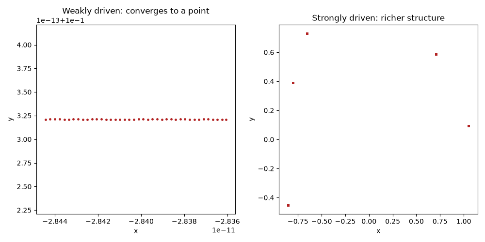
Sampling the Duffing oscillator’s state once per drive period (stroboscopically) collapses its effectively-3D state space (position, velocity, and drive phase) back to a 2D picture: a periodic response shows up as one (or a few) fixed points, while chaotic parameters produce a scattered, fractal-looking set of points.

import matplotlib.pyplot as plt

from mathematicskit.ode_dynamics.systems.poincare import DuffingOscillator, stroboscopic_poincare_section
from mathematicskit.ode_dynamics.visualizers.plots import plot_poincare_points

A weakly driven system settles onto a single periodic point

system_periodic = DuffingOscillator([0.1, 0.0], delta=0.5, alpha=1.0, beta=0.0, gamma=0.05, omega=1.0)
xs_p, ys_p = stroboscopic_poincare_section(system_periodic, n_periods=40, n_transient_periods=40, dt=1e-2)

A more strongly driven double-well system shows a richer section

system_rich = DuffingOscillator([1.0, 0.0], delta=0.3, alpha=-1.0, beta=1.0, gamma=0.37, omega=1.2)
xs_r, ys_r = stroboscopic_poincare_section(system_rich, n_periods=400, n_transient_periods=200, dt=1e-2)

fig, axes = plt.subplots(1, 2, figsize=(10, 5))
plot_poincare_points(xs_p, ys_p, ax=axes[0])
axes[0].set_title("Weakly driven: converges to a point")
plot_poincare_points(xs_r, ys_r, ax=axes[1])
axes[1].set_title("Strongly driven: richer structure")
fig.tight_layout()

plt.show()