Lotka-Volterra predator-prey cycles

Predator and prey populations rise and fall periodically, out of phase. Every orbit is closed because the Lotka-Volterra invariant \(V = \delta x - \gamma\ln x + \beta y - \alpha\ln y\) is conserved: orbits are its level sets around the coexistence fixed point.

import matplotlib.pyplot as plt
import numpy as np

from mathematicskit.ode_dynamics.systems.population import LotkaVolterra, lotka_volterra_invariant

params = dict(alpha=1.1, beta=0.4, delta=0.1, gamma=0.4)

Nested closed orbits and out-of-phase oscillations

fig, axes = plt.subplots(1, 2, figsize=(11, 4.5))
for x0 in (5.0, 10.0, 20.0):
    system = LotkaVolterra([x0, 2.75], **params)
    traj = system.integrate((0.0, 40.0), dt=1e-3, method="rk4")
    axes[0].plot(traj.y[:, 0], traj.y[:, 1], lw=1)
    V = lotka_volterra_invariant(traj.y[:, 0], traj.y[:, 1], **params)
    print(f"x0={x0:5.1f}: invariant drift over t=40 is {np.ptp(V):.1e}")
fp = system.fixed_point()
axes[0].plot(*fp, "k+", ms=12, label="coexistence fixed point")
axes[0].set_xlabel("prey x")
axes[0].set_ylabel("predators y")
axes[0].set_title("Orbits are level sets of the invariant")
axes[0].legend()

axes[1].plot(traj.t, traj.y[:, 0], label="prey")
axes[1].plot(traj.t, traj.y[:, 1], label="predators")
axes[1].set_xlabel("t")
axes[1].set_title("Predator peaks lag prey peaks")
axes[1].legend()
fig.tight_layout()

plt.show()

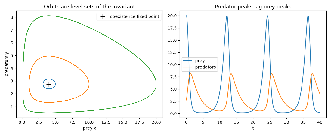
x0=  5.0: invariant drift over t=40 is 2.7e-15
x0= 10.0: invariant drift over t=40 is 1.4e-14
x0= 20.0: invariant drift over t=40 is 3.4e-13