Dahlquist’s A-stability: backward Euler vs RK4

Applied to the test equation \(y' = \lambda y\), a one-step method multiplies \(y\) by a stability function \(R(z)\), with \(z = \lambda h\). Dahlquist (1963) called a method A-stable if \(|R(z)| \le 1\) on the whole left half-plane, so that no decaying mode can ever be amplified, whatever the step size. Explicit methods never qualify, since their \(R\) is a polynomial and grows without bound. RK4’s region reaches only \(z \approx -2.785\) on the real axis. Backward Euler’s \(R(z) = 1/(1 - z)\) is A-stable. Dahlquist also proved that no A-stable linear multistep method can exceed order 2 (his “second barrier”).

import matplotlib.pyplot as plt
import numpy as np

from mathematicskit.integrators import implicit_euler_integrate, is_absolutely_stable, njit, rk4_integrate
from mathematicskit.ode_dynamics.visualizers import plot_stability_regions

Stability regions in the complex z-plane

fig, axes = plt.subplots(1, 3, figsize=(14, 4.2))
for ax, (method, name) in zip(axes[:2], [("rk4", "RK4"), ("implicit_euler", "backward Euler")], strict=True):
    plot_stability_regions(method, ax=ax, re_range=(-5, 3), im_range=(-4, 4), labels=[name])
    ax.set_title(f"{name}: shaded where |R(z)| <= 1")

x, y = np.meshgrid(np.linspace(-50, 0, 201), np.linspace(-50, 50, 401))
left_half_plane = x + 1j * y
for method in ("rk4", "implicit_euler"):
    print(f"{method}: stable on the whole sampled left half-plane? {is_absolutely_stable(method, left_half_plane).all()}")

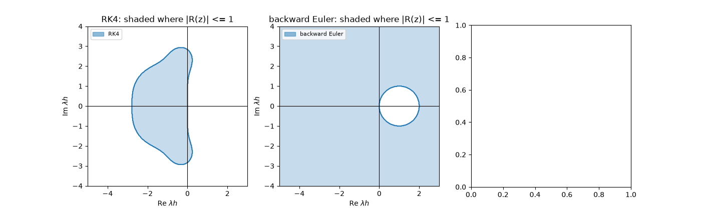
rk4: stable on the whole sampled left half-plane? False
implicit_euler: stable on the whole sampled left half-plane? True

Consequence on a stiff equation, lambda * h = 30

The Prothero-Robinson equation \(y' = -\lambda(y - \cos t) - \sin t\) has the smooth solution \(y = \cos t\), but with \(\lambda = 3000\) and \(h = 0.01\), \(z = -30\) lies far outside RK4’s region.

@njit
def prothero_robinson(state, t, params):
    return -params[0] * (state - np.cos(t)) - np.sin(t)


params = np.array([3000.0])
ts, ys_ie = implicit_euler_integrate(prothero_robinson, np.array([1.0]), 0.0, 1e-2, 40, params)
_, ys_rk4 = rk4_integrate(prothero_robinson, np.array([1.0]), 0.0, 1e-2, 40, params)
axes[2].semilogy(ts, np.abs(ys_rk4[:, 0] - np.cos(ts)) + 1e-16, "o-", ms=3, label="RK4")
axes[2].semilogy(ts, np.abs(ys_ie[:, 0] - np.cos(ts)) + 1e-16, "s-", ms=3, label="backward Euler")
axes[2].set_xlabel("t")
axes[2].set_ylabel("|error|")
axes[2].set_title("z = -30: only the A-stable method survives")
axes[2].legend()
fig.tight_layout()

print(f"final error: RK4 {abs(ys_rk4[-1, 0] - np.cos(ts[-1])):.2e}, backward Euler {abs(ys_ie[-1, 0] - np.cos(ts[-1])):.2e}")

plt.show()

final error: RK4 7.41e+172, backward Euler 1.54e-06