Curtiss and Hirschfelder: stiffness and BDF

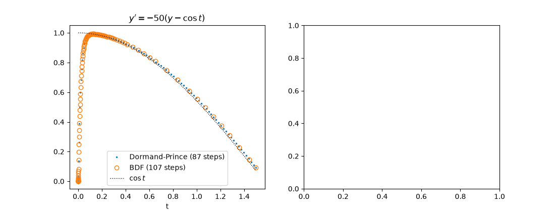
Curtiss and Hirschfelder (1952) named the difficulty “stiffness” while integrating chemical-kinetics equations, using the model problem

\[y' = -\lambda\,(y - \cos t),\qquad \lambda = 50.\]

After a transient lasting about \(1/\lambda\), \(y\) follows the slow curve \(\approx \cos t\), yet an explicit method’s step stays pinned near \(1/\lambda\). Their remedy was the backward differentiation formulas (BDF), which fit a polynomial through past values and require it to satisfy the ODE at the new point. BDF1 is backward Euler, and BDF2 is \(\tfrac32 y_{n+1} - 2y_n + \tfrac12 y_{n-1} = h f(t_{n+1}, y_{n+1})\). Gear (1971) turned them into variable-order codes, and stiff_integrate() with method="BDF" is a descendant.

import matplotlib.pyplot as plt
import numpy as np

from mathematicskit.integrators import dopri5_integrate, njit, stiff_integrate


@njit
def curtiss_hirschfelder(state, t, params):
    return -params[0] * (state - np.cos(t))


state0 = np.array([0.0])
t_end = 1.5

The 1952 problem, lambda = 50

params = np.array([50.0])
ts_bdf, ys_bdf = stiff_integrate(curtiss_hirschfelder, state0, 0.0, t_end, params, method="BDF", rtol=1e-6, atol=1e-9)
ts_dp, ys_dp = dopri5_integrate(curtiss_hirschfelder, state0, 0.0, t_end, 1e-4, params, rtol=1e-6, atol=1e-9)

fig, (ax0, ax1) = plt.subplots(1, 2, figsize=(11, 4.2))
ax0.plot(ts_dp, ys_dp[:, 0], ".", ms=3, label=f"Dormand-Prince ({len(ts_dp) - 1} steps)")
ax0.plot(ts_bdf, ys_bdf[:, 0], "o", mfc="none", label=f"BDF ({len(ts_bdf) - 1} steps)")
ax0.plot(ts_dp, np.cos(ts_dp), "k:", lw=1, label=r"$\cos t$")
ax0.set_xlabel("t")
ax0.set_title(r"$y' = -50(y - \cos t)$")
ax0.legend()

<matplotlib.legend.Legend object at 0x7fd7c5a35430>

Explicit cost grows with lambda, BDF’s does not

lams = np.array([50.0, 500.0, 5000.0, 50000.0])
steps_dp, steps_bdf = [], []
for lam in lams:
    p = np.array([lam])
    steps_dp.append(len(dopri5_integrate(curtiss_hirschfelder, state0, 0.0, t_end, 1e-5, p, rtol=1e-6, atol=1e-9)[0]) - 1)
    steps_bdf.append(len(stiff_integrate(curtiss_hirschfelder, state0, 0.0, t_end, p, method="BDF", rtol=1e-6, atol=1e-9)[0]) - 1)
    print(f"lambda={lam:>8.0f}: Dormand-Prince {steps_dp[-1]:6d} steps, BDF {steps_bdf[-1]:4d} steps")

ax1.loglog(lams, steps_dp, "o-", label="Dormand-Prince (explicit)")
ax1.loglog(lams, steps_bdf, "s-", label="BDF (implicit)")
ax1.set_xlabel(r"stiffness $\lambda$")
ax1.set_ylabel("accepted steps")
ax1.set_title("Stiffness: cost set by stability, not accuracy")
ax1.legend()
fig.tight_layout()

plt.show()

lambda=      50: Dormand-Prince     89 steps, BDF  107 steps
lambda=     500: Dormand-Prince    343 steps, BDF  124 steps
lambda=    5000: Dormand-Prince   2316 steps, BDF  118 steps
lambda=   50000: Dormand-Prince  22693 steps, BDF  122 steps