Butcher, Ehle and Radau IIA: L-stable implicit Runge-Kutta

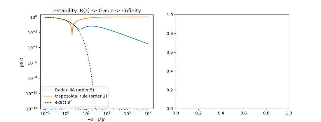
Butcher (1964) built implicit Runge-Kutta methods on Gauss and Radau quadrature nodes. Ehle (1969) showed that their stability functions are Padé approximants of \(e^z\), and that the Radau IIA family is A-stable and, moreover, L-stable: \(R(z) \to 0\) as \(z \to -\infty\), so infinitely stiff modes are damped in a single step. The three-stage, order-5 method used by stiff_integrate() has

\[R(z) = \frac{1 + \tfrac25 z + \tfrac1{20} z^2} {1 - \tfrac35 z + \tfrac3{20} z^2 - \tfrac1{60} z^3}.\]

The trapezoidal rule is A-stable but not L-stable, since \(R(z) \to -1\): stiff components flip sign each step instead of dying.

import matplotlib.pyplot as plt
import numpy as np

from mathematicskit.integrators import njit, stiff_integrate

Damping of stiff modes

z = -np.logspace(-1, 4, 300)
r_radau = (1 + 2 * z / 5 + z**2 / 20) / (1 - 3 * z / 5 + 3 * z**2 / 20 - z**3 / 60)
r_trap = (1 + z / 2) / (1 - z / 2)

fig, (ax0, ax1) = plt.subplots(1, 2, figsize=(11, 4.2))
ax0.loglog(-z, np.abs(r_radau), label="Radau IIA (order 5)")
ax0.loglog(-z, np.abs(r_trap), label="trapezoidal rule (order 2)")
ax0.loglog(-z, np.exp(z).clip(1e-30), "k:", label=r"exact $e^{z}$")
ax0.set_ylim(1e-12, 2)
ax0.set_xlabel(r"$-z = |\lambda| h$")
ax0.set_ylabel(r"$|R(z)|$")
ax0.set_title("L-stability: R(z) -> 0 as z -> -infinity")
ax0.legend()

<matplotlib.legend.Legend object at 0x7fd7c3149d00>

The stiff van der Pol oscillator, mu = 1000

Relaxation oscillations with slow drifts and near-instant jumps. This is the classic stiff Radau IIA benchmark (Hairer and Wanner). Over \(0 \le t \le 3000\) Radau IIA needs about 1200 steps; scipy’s explicit RK45 needs about 1.7 million at the same tolerance.

@njit
def van_der_pol(state, t, params):
    mu = params[0]
    return np.array([state[1], mu * (1 - state[0] ** 2) * state[1] - state[0]])


ts, ys = stiff_integrate(van_der_pol, np.array([2.0, 0.0]), 0.0, 3000.0, np.array([1000.0]), method="Radau", rtol=1e-6, atol=1e-8)
ax1.plot(ts, ys[:, 0], "-", lw=1)
ax1.plot(ts, ys[:, 0], ".", ms=2)
ax1.set_xlabel("t")
ax1.set_ylabel("x")
ax1.set_title(f"Radau IIA on van der Pol, mu = 1000 ({len(ts) - 1} steps)")
fig.tight_layout()

print(f"Radau IIA: {len(ts) - 1} steps; smallest step {np.min(np.diff(ts)):.1e}, largest {np.max(np.diff(ts)):.1e}")

plt.show()

Radau IIA: 1187 steps; smallest step 3.9e-05, largest 1.1e+02