De Boor and Swartz: collocation for boundary-value problems

A two-point boundary-value problem fixes conditions at both ends, so there is no initial state to march forward from. Collocation solves for the whole solution at once. It takes a piecewise polynomial on a mesh and requires it to satisfy the ODE exactly at a few collocation points per interval and to meet the boundary conditions, which gives one nonlinear system for Newton’s method. De Boor and Swartz (1973) proved that collocation with \(k\) Gauss points per interval converges with order \(2k\) at the mesh nodes (“superconvergence”). This made it the basis of BVP codes such as COLSYS and scipy.integrate.solve_bvp(), which uses the closely related 3-point Lobatto IIIA scheme.

Bratu’s problem (1914), \(y'' + \lambda e^{y} = 0\) with \(y(0) = y(1) = 0\), has two solutions for \(0 < \lambda < \lambda_c \approx 3.51\), and the initial guess picks which one Newton converges to. Both are known in closed form, \(y = -2\ln\!\big[\cosh((x - \tfrac12)\theta/2) / \cosh(\theta/4)\big]\) with \(\theta = \sqrt{2\lambda}\cosh(\theta/4)\).

import matplotlib.pyplot as plt
import numpy as np
from scipy.optimize import fsolve

from mathematicskit.integrators import collocation_bvp, njit


@njit
def bratu(state, x, params):
    out = np.empty(2)
    out[0] = state[1]
    out[1] = -params[0] * np.exp(state[0])
    return out


def dirichlet_zero(ya, yb, params):
    return np.array([ya[0], yb[0]])


lam = 1.0
params = np.array([lam])
x = np.linspace(0.0, 1.0, 11)

Two initial guesses, two solutions

guesses = {
    "guess y = 0": np.zeros((x.size, 2)),
    "guess y = 4 sin(pi x)": np.column_stack([4 * np.sin(np.pi * x), 4 * np.pi * np.cos(np.pi * x)]),
}
xq = np.linspace(0.0, 1.0, 200)
fig, ax = plt.subplots(figsize=(7, 4.5))
for (label, guess), theta0 in zip(guesses.items(), (1.5, 10.0), strict=False):
    res = collocation_bvp(bratu, dirichlet_zero, x, guess, params, tol=1e-8)
    theta = fsolve(lambda th: th - np.sqrt(2 * lam) * np.cosh(th / 4), theta0)[0]
    exact = -2 * np.log(np.cosh((xq - 0.5) * theta / 2) / np.cosh(theta / 4))
    ax.plot(xq, res.sol(xq)[:, 0], lw=2, label=f"{label} ({res.x.size} nodes)")
    ax.plot(xq, exact, "k:", lw=1)
    print(f"{label}: success={res.success}, max |error| = {np.max(np.abs(res.sol(xq)[:, 0] - exact)):.2e}")

ax.set_xlabel("x")
ax.set_ylabel("y")
ax.set_title(r"Collocation on Bratu, $\lambda = 1$ (solid) vs exact (dotted)")
ax.legend()
fig.tight_layout()

plt.show()

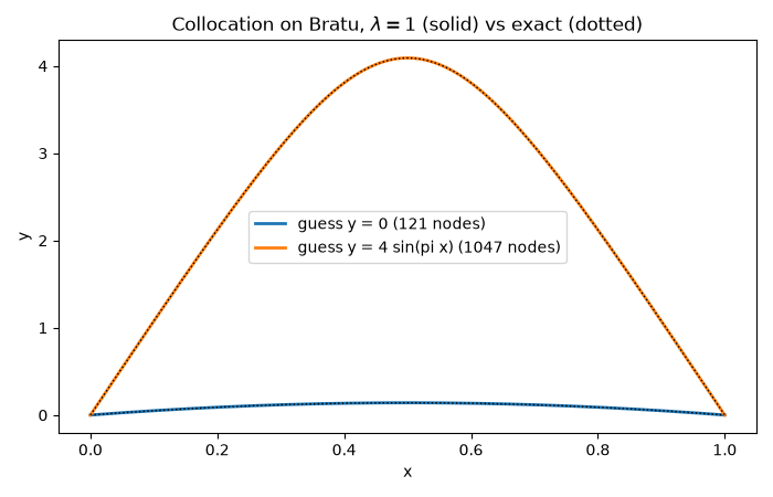
guess y = 0: success=True, max |error| = 2.18e-11
guess y = 4 sin(pi x): success=True, max |error| = 4.15e-11