The Kuramoto synchronization transition

A thousand oscillators with Lorentzian-distributed natural frequencies stay incoherent for weak coupling. Above the critical coupling \(K_c = 2\gamma\) a synchronized cluster forms, and the steady coherence follows Kuramoto’s exact result \(r = \sqrt{1 - K_c/K}\).

import matplotlib.pyplot as plt
import numpy as np

from mathematicskit.ode_dynamics.systems.synchronization import KuramotoModel, kuramoto_lorentzian_order_parameter, kuramoto_order_parameter

n, gamma = 1000, 0.5
omegas = gamma * np.tan(np.pi * (np.arange(n) + 0.5) / n - np.pi / 2)
theta0 = np.random.default_rng(0).uniform(0.0, 2.0 * np.pi, n)

Coherence versus coupling strength

Ks = np.linspace(0.25, 4.0, 16)
r_sim = []
for K in Ks:
    traj = KuramotoModel(theta0, omegas, K=K).integrate((0.0, 60.0), dt=0.02, method="rk4")
    r_sim.append(kuramoto_order_parameter(traj.y[-500:])[0].mean())
K_fine = np.linspace(0.25, 4.0, 300)

fig, axes = plt.subplots(1, 2, figsize=(11, 4.5))
axes[0].plot(K_fine, kuramoto_lorentzian_order_parameter(K_fine, gamma), "k", label="theory sqrt(1 - Kc/K)")
axes[0].plot(Ks, r_sim, "o", label=f"simulation, N={n}")
axes[0].axvline(2 * gamma, color="gray", ls="--")
axes[0].set_xlabel("coupling K")
axes[0].set_ylabel("order parameter r")
axes[0].set_title("Onset of synchrony at Kc = 2 gamma")
axes[0].legend()

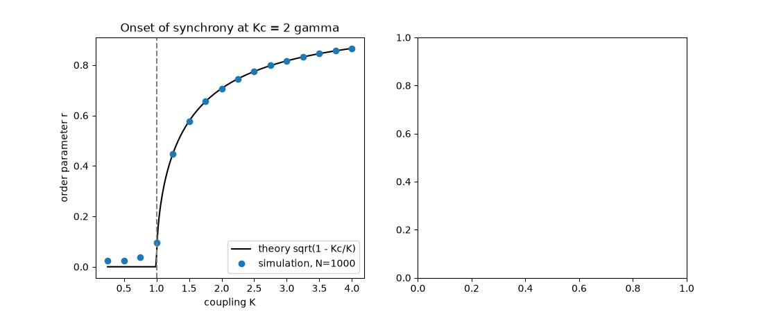
<matplotlib.legend.Legend object at 0x1192fa510>

Growth of coherence over time

for K in (0.5, 1.5, 3.0):
    traj = KuramotoModel(theta0, omegas, K=K).integrate((0.0, 30.0), dt=0.02, method="rk4")
    axes[1].plot(traj.t, kuramoto_order_parameter(traj.y)[0], label=f"K={K}")
axes[1].set_xlabel("t")
axes[1].set_ylabel("r(t)")
axes[1].set_title("Coherence r(t)")
axes[1].legend()
fig.tight_layout()

plt.show()