Kirkpatrick, Gelatt and Vecchi’s simulated annealing

Gradient methods slide into the nearest valley. Kirkpatrick, Gelatt and Vecchi (1983) borrowed the Metropolis rule from statistical physics: accept any downhill move, and an uphill move of size \(\Delta f\) with probability \(e^{-\Delta f/T}\), while the temperature \(T\) is lowered slowly, as in annealing a metal.

Rastrigin’s function \(f(x) = 10n + \sum_i (x_i^2 - 10\cos 2\pi x_i)\) has a local minimum near every integer point and its global minimum \(f = 0\) at the origin.

import matplotlib.pyplot as plt
import numpy as np
from scipy import optimize

from mathematicskit.optimization import GradientDescentLineSearch, simulated_annealing


def rastrigin(x):
    x = np.asarray(x)
    return 10 * x.shape[0] + np.sum(x**2 - 10 * np.cos(2 * np.pi * x), axis=0)


def rastrigin_grad(x):
    return 2 * x + 20 * np.pi * np.sin(2 * np.pi * x)

In two dimensions: descent gets trapped, annealing does not

x0 = np.array([4.4, -3.6])
descent = GradientDescentLineSearch(tol=1e-8).minimize(rastrigin, rastrigin_grad, x0)
annealed = simulated_annealing(lambda x: float(rastrigin(x)), x0, step_size=0.4, t0=20.0, cooling=0.9995, n_iter=15000, seed=3)
reference = optimize.dual_annealing(lambda x: float(rastrigin(x)), bounds=[(-5.12, 5.12)] * 2, seed=0)
print(f"gradient descent      : x = {descent.x.round(3)}, f = {descent.fun:.3f}  (a local minimum)")
print(f"simulated annealing   : x = {annealed.x.round(3)}, f = {annealed.fun:.4f}")
print(f"scipy dual_annealing  : x = {reference.x.round(3)}, f = {reference.fun:.4f}")

grid = np.linspace(-5.12, 5.12, 300)
gx, gy = np.meshgrid(grid, grid)
fig, (ax0, ax1) = plt.subplots(1, 2, figsize=(13, 5.2))
ax0.contourf(gx, gy, rastrigin(np.array([gx, gy])), levels=30, cmap="Greys")
ax0.plot(*annealed.path[::10].T, "-", color="tab:orange", lw=0.6, alpha=0.8, label="simulated annealing")
ax0.plot(*descent.path.T, "o-", color="tab:blue", ms=3, label="gradient descent")
ax0.plot(*x0, "k^", ms=10, label="start")
ax0.plot(0, 0, "r*", ms=14, label="global minimum")
ax0.set_aspect("equal")
ax0.legend(loc="lower left", fontsize=8)
ax0.set_title("Rastrigin's function in 2D")

ax1.semilogy(annealed.extra["energies"] + 1e-3, lw=0.7, color="tab:orange", label="f(current state) + 0.001")
ax1.semilogy(annealed.extra["temperatures"], "k--", lw=1, label="temperature T")
ax1.set_xlabel("step")
ax1.set_title("The energy follows the temperature down")
ax1.legend(fontsize=8)
fig.tight_layout()

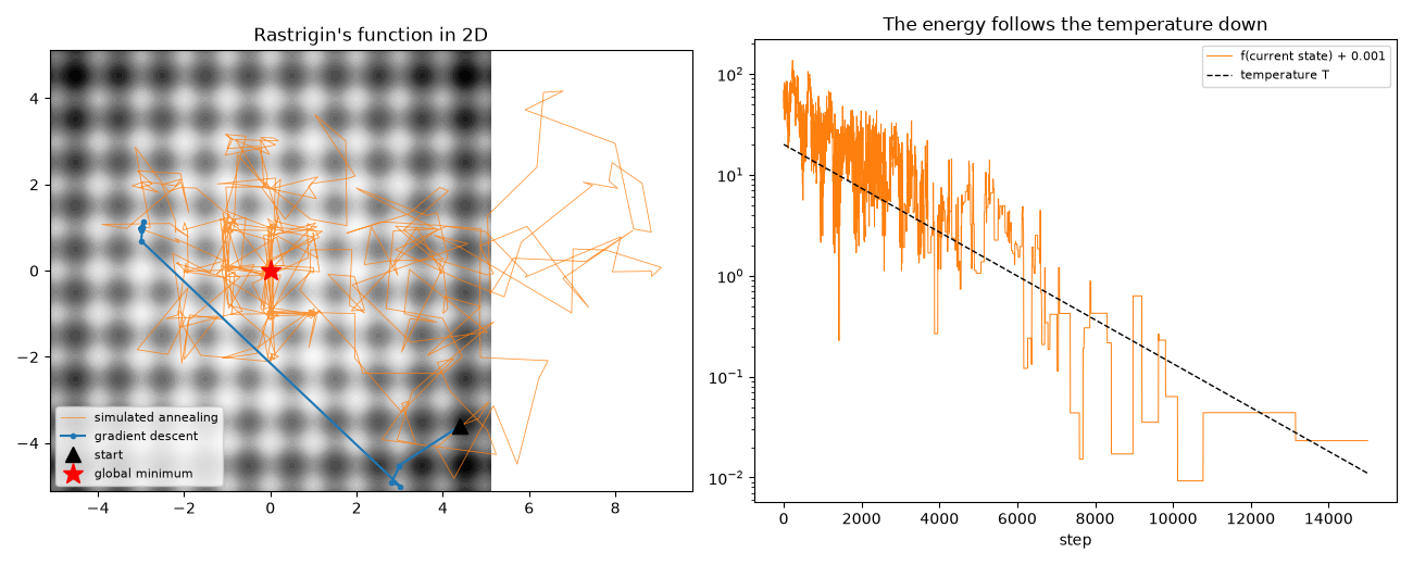
gradient descent      : x = [-2.985  0.995], f = 9.950  (a local minimum)
simulated annealing   : x = [0.002 0.006], f = 0.0083
scipy dual_annealing  : x = [-0. -0.], f = 0.0000

In eight dimensions: the cooling schedule matters

With \(T = 0\) (a “quench”) the method only accepts downhill moves and stops in a high local minimum. Cooling more slowly lets the walk cross more barriers before it freezes, and ends lower. Each schedule is run from the same start with eight different random seeds.

x0_8d = np.full(8, 3.5)
schedules = {"quench (T = 0)": lambda k: 0.0, "fast, 0.99^k": 0.99, "medium, 0.999^k": 0.999, "slow, 0.9997^k": 0.9997}
finals = {}
for name, cooling in schedules.items():
    runs = [simulated_annealing(lambda x: float(rastrigin(x)), x0_8d, step_size=0.3, t0=30.0, cooling=cooling, n_iter=20000, seed=s) for s in range(8)]
    finals[name] = [r.fun for r in runs]
    print(f"{name:16s}: best f over 8 runs = {min(finals[name]):6.2f}, median {np.median(finals[name]):6.2f}")

fig, ax = plt.subplots(figsize=(7, 4))
for k, values in enumerate(finals.values()):
    ax.plot(np.full(len(values), k) + np.linspace(-0.1, 0.1, len(values)), values, "o", alpha=0.7)
ax.set_xticks(range(len(finals)), list(finals))
ax.set_ylabel("final f (global minimum 0)")
ax.set_title("8-D Rastrigin: slower cooling finds deeper minima")
fig.tight_layout()

plt.show()

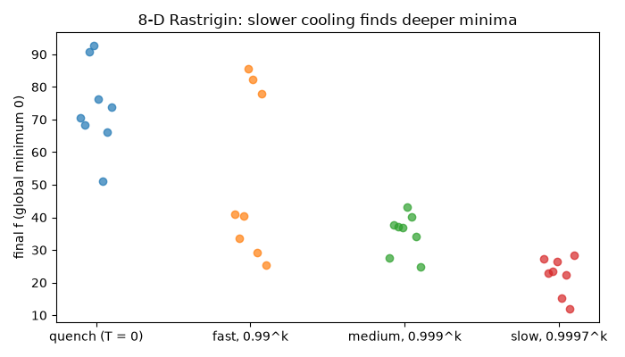
quench (T = 0)  : best f over 8 runs =  50.97, median  72.18
fast, 0.99^k    : best f over 8 runs =  25.24, median  40.65
medium, 0.999^k : best f over 8 runs =  24.73, median  37.07
slow, 0.9997^k  : best f over 8 runs =  11.91, median  23.14