Lagrange multipliers and the KKT conditions

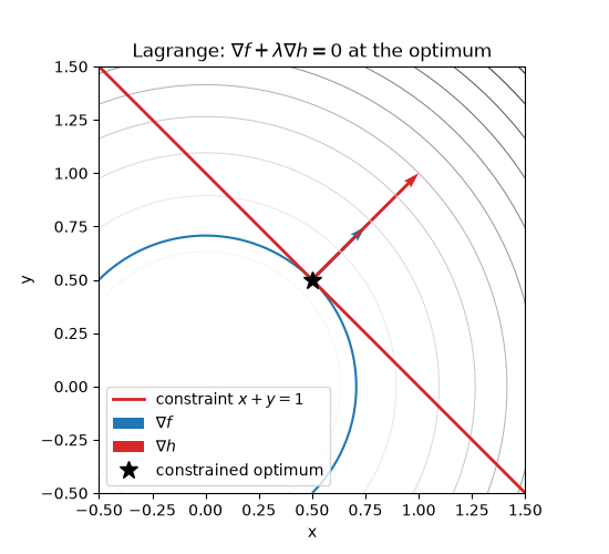
Minimizes \(x^2+y^2\) subject to \(x+y=1\). At the constrained optimum \((0.5, 0.5)\) the objective’s gradient is parallel to the constraint’s gradient, \(\nabla f = -\lambda \nabla h\) with \(\lambda=-1\), which is Lagrange’s condition. Rewriting the constraint as the inequality \(x+y \geq 1\) gives a Karush-Kuhn-Tucker problem whose multiplier must also be non-negative.

import matplotlib.pyplot as plt
import numpy as np

from mathematicskit.optimization import lagrange_stationary_point, verify_kkt

f = lambda z: z[0] ** 2 + z[1] ** 2
grad_f = lambda z: np.array([2.0 * z[0], 2.0 * z[1]])
h = lambda z: np.array([z[0] + z[1] - 1.0])
grad_h = lambda z: np.array([[1.0, 1.0]])

Solve the Lagrange stationarity system

The unknowns are \((x, y, \lambda)\): \(\nabla f + \lambda \nabla h = 0\) and \(h = 0\).

lagrange = lagrange_stationary_point(grad_f, h, grad_h, x0=np.array([0.0, 0.0]))
x_star, lam = lagrange.x, lagrange.multipliers
print(f"x* = {x_star.round(6)}, lambda* = {lam.round(6)}")
print(f"grad f(x*) = {grad_f(x_star).round(6)}, -lambda * grad h = {(-lam[0] * grad_h(x_star)[0]).round(6)}")

x* = [0.5 0.5], lambda* = [-1.]
grad f(x*) = [1. 1.], -lambda * grad h = [1. 1.]

Gradients are parallel at the constrained optimum

xs = np.linspace(-0.5, 1.5, 200)
X, Y = np.meshgrid(xs, xs)
fig, ax = plt.subplots(figsize=(5.5, 5))
ax.contour(X, Y, X**2 + Y**2, levels=12, cmap="Greys", linewidths=0.7)
ax.contour(X, Y, X**2 + Y**2, levels=[f(x_star)], colors="tab:blue", linewidths=1.5)
ax.plot(xs, 1.0 - xs, color="tab:red", lw=2, label=r"constraint $x + y = 1$")
ax.quiver(*x_star, *(0.25 * grad_f(x_star)), color="tab:blue", angles="xy", scale_units="xy", scale=1, label=r"$\nabla f$")
ax.quiver(*x_star, *(0.5 * grad_h(x_star)[0]), color="tab:red", angles="xy", scale_units="xy", scale=1, label=r"$\nabla h$")
ax.plot(*x_star, "k*", ms=12, label="constrained optimum")
ax.set_xlim(-0.5, 1.5)
ax.set_ylim(-0.5, 1.5)
ax.set_aspect("equal")
ax.set_xlabel("x")
ax.set_ylabel("y")
ax.legend(loc="lower left")
ax.set_title(r"Lagrange: $\nabla f + \lambda \nabla h = 0$ at the optimum")

Text(0.5, 1.0, 'Lagrange: $\\nabla f + \\lambda \\nabla h = 0$ at the optimum')

Verify the KKT conditions

For the equality constraint, stationarity and feasibility are all that is needed. As an inequality \(g(x) = 1 - x - y \leq 0\), the KKT conditions also require dual feasibility \(\mu \geq 0\) and complementary slackness \(\mu g(x) = 0\): here \(\mu = 1\) certifies the optimum, while the wrong-sign multiplier \(\mu = -1\) does not.

kkt_eq = verify_kkt(x_star, grad_f, h=h, grad_h=grad_h, eq_multipliers=lam)
print(f"equality form:   KKT satisfied = {kkt_eq.satisfied}, stationarity residual = {kkt_eq.stationarity_residual:.1e}")

g = lambda z: np.array([1.0 - z[0] - z[1]])
grad_g = lambda z: np.array([[-1.0, -1.0]])
for mu in (1.0, -1.0):
    kkt = verify_kkt(x_star, grad_f, g=g, grad_g=grad_g, ineq_multipliers=np.array([mu]))
    print(f"inequality form, mu = {mu:+.0f}: satisfied = {kkt.satisfied}, dual feasible = {kkt.dual_feasible}")

equality form:   KKT satisfied = True, stationarity residual = 0.0e+00
inequality form, mu = +1: satisfied = True, dual feasible = True
inequality form, mu = -1: satisfied = False, dual feasible = False