The quadratic penalty method: a sequence of unconstrained problems

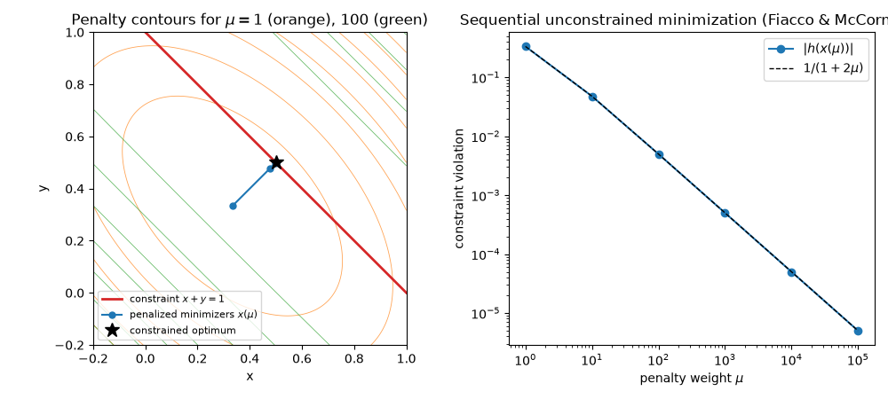
Fiacco and McCormick’s sequential unconstrained minimization replaces \(\min x^2+y^2\) subject to \(x+y=1\) with the unconstrained problems \(\min x^2+y^2+\mu(x+y-1)^2\) for growing \(\mu\). Each penalized minimizer violates the constraint slightly, and the violation shrinks like \(1/\mu\) as the minimizers approach the constrained optimum \((0.5, 0.5)\).

import matplotlib.pyplot as plt
import numpy as np

from mathematicskit.optimization import PenaltyMethod

f = lambda z: z[0] ** 2 + z[1] ** 2
grad_f = lambda z: np.array([2.0 * z[0], 2.0 * z[1]])
h = lambda z: np.array([z[0] + z[1] - 1.0])
grad_h = lambda z: np.array([[1.0, 1.0]])

Solve the penalized problems for \(\mu = 1, 10, 100, \ldots\)

Running the method with one more outer iteration each time exposes the minimizer of every subproblem. The exact penalized minimizer is \(x = y = \mu/(1+2\mu)\).

x0 = np.array([0.0, 0.0])
mus, minimizers = [], []
for n_outer in range(1, 7):
    result = PenaltyMethod(mu0=1.0, mu_factor=10.0, n_outer=n_outer).minimize(f, grad_f, x0, h=h, grad_h=grad_h)
    mus.append(result.extra["mu_history"][-1])
    minimizers.append(result.x)
mus, minimizers = np.array(mus), np.array(minimizers)
violation = np.abs(minimizers.sum(axis=1) - 1.0)
for mu, x, v in zip(mus, minimizers, violation):
    print(f"mu = {mu:>8.0f}: x = {x.round(6)}, exact {mu / (1 + 2 * mu):.6f}, |h(x)| = {v:.1e}")

mu =        1: x = [0.333333 0.333333], exact 0.333333, |h(x)| = 3.3e-01
mu =       10: x = [0.47619 0.47619], exact 0.476190, |h(x)| = 4.8e-02
mu =      100: x = [0.497512 0.497512], exact 0.497512, |h(x)| = 5.0e-03
mu =     1000: x = [0.49975 0.49975], exact 0.499750, |h(x)| = 5.0e-04
mu =    10000: x = [0.499975 0.499975], exact 0.499975, |h(x)| = 5.0e-05
mu =   100000: x = [0.499998 0.499998], exact 0.499998, |h(x)| = 5.0e-06

Minimizers approach the constraint; violation falls like 1/mu

fig, (ax1, ax2) = plt.subplots(1, 2, figsize=(10, 4.5))
xs = np.linspace(-0.2, 1.0, 200)
X, Y = np.meshgrid(xs, xs)
for mu, color in zip((1.0, 100.0), ("tab:orange", "tab:green")):
    ax1.contour(X, Y, X**2 + Y**2 + mu * (X + Y - 1.0) ** 2, levels=8, colors=color, linewidths=0.6, alpha=0.7)
ax1.plot(xs, 1.0 - xs, color="tab:red", lw=2, label=r"constraint $x + y = 1$")
ax1.plot(*minimizers.T, "o-", color="tab:blue", ms=5, label=r"penalized minimizers $x(\mu)$")
ax1.plot(0.5, 0.5, "k*", ms=12, label="constrained optimum")
ax1.set_xlim(-0.2, 1.0)
ax1.set_ylim(-0.2, 1.0)
ax1.set_aspect("equal")
ax1.set_xlabel("x")
ax1.set_ylabel("y")
ax1.legend(loc="lower left", fontsize=8)
ax1.set_title(r"Penalty contours for $\mu = 1$ (orange), $100$ (green)")
ax2.loglog(mus, violation, "o-", label=r"$|h(x(\mu))|$")
ax2.loglog(mus, 1.0 / (1.0 + 2.0 * mus), "k--", lw=1, label=r"$1/(1+2\mu)$")
ax2.set_xlabel(r"penalty weight $\mu$")
ax2.set_ylabel("constraint violation")
ax2.legend()
ax2.set_title("Sequential unconstrained minimization (Fiacco & McCormick)")
fig.tight_layout()