Levenberg-Marquardt: fitting a damped oscillation

Fits a four-parameter damped cosine to noisy data. The residuals depend nonlinearly on the decay rate and frequency, so the fit needs an iterative method; Levenberg-Marquardt blends gradient descent (far from the solution) with Gauss-Newton (close to it).

import matplotlib.pyplot as plt
import numpy as np

from mathematicskit.optimization import levenberg_marquardt

Noisy data from a known model

rng = np.random.default_rng(0)
t = np.linspace(0.0, 10.0, 120)
true = np.array([2.0, 0.3, 1.5, 0.4])  # amplitude, decay, frequency, phase


def model(p, t):
    return p[0] * np.exp(-p[1] * t) * np.cos(p[2] * t + p[3])


y = model(true, t) + 0.05 * rng.normal(size=t.size)

Fit from a rough initial guess

x0 = [1.0, 0.1, 1.3, 0.0]
result = levenberg_marquardt(lambda p: model(p, t) - y, x0)
print(f"true parameters:   {true}")
print(f"fitted parameters: {result.x.round(4)}")
print(f"residual cost 0.5*||r||^2 = {result.cost:.4f} after {result.nfev} evaluations")

fig, ax = plt.subplots()
ax.plot(t, y, ".", color="0.5", label="data")
ax.plot(t, model(x0, t), "--", label="initial guess")
ax.plot(t, model(result.x, t), label="Levenberg-Marquardt fit")
ax.set_xlabel("t")
ax.legend()
ax.set_title("Nonlinear least squares (Levenberg 1944, Marquardt 1963)")

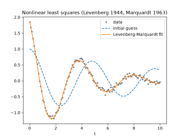
true parameters:   [2.  0.3 1.5 0.4]
fitted parameters: [2.0297 0.3011 1.5011 0.4084]
residual cost 0.5*||r||^2 = 0.1332 after 8 evaluations

Text(0.5, 1.0, 'Nonlinear least squares (Levenberg 1944, Marquardt 1963)')