The travelling salesman: Held and Karp’s exact algorithm

A salesman must visit \(n\) cities and return home by the shortest route. Trying all \((n-1)!/2\) tours is hopeless beyond a dozen cities; Held and Karp (1962) found the optimum in \(O(n^2 2^n)\) steps by dynamic programming over the set of cities visited so far, still the best worst-case bound known. Heuristics are faster but inexact: the nearest-neighbour tour, and Croes’s 2-opt move, which reverses a segment whenever that removes a crossing.

import math
import time

import matplotlib.pyplot as plt
import numpy as np

from mathematicskit.optimization import distance_matrix, tsp_held_karp, tsp_nearest_neighbor, tsp_two_opt

cities = np.random.default_rng(1962).uniform(size=(14, 2))
dist = distance_matrix(cities)
n = len(cities)
print(f"{n} cities: {math.factorial(n - 1) // 2:,} distinct tours, Held-Karp table of {n * 2 ** (n - 1):,} entries")

14 cities: 3,113,510,400 distinct tours, Held-Karp table of 114,688 entries

Three tours

start = time.perf_counter()
exact = tsp_held_karp(dist)
elapsed = time.perf_counter() - start
nearest = tsp_nearest_neighbor(dist)
improved = tsp_two_opt(dist, nearest.tour)
for result in (nearest, improved, exact):
    print(f"{result.method:16s} length {result.length:.4f} ({100 * (result.length / exact.length - 1):5.2f}% above optimal)")
print(f"Held-Karp took {elapsed:.2f} s")

fig, axes = plt.subplots(1, 3, figsize=(15, 5))
for ax, result, title in zip(
    axes,
    (nearest, improved, exact),
    ("Nearest neighbour", f"2-opt ({len(improved.history) - 1} improving moves)", "Held-Karp: optimal"),
    strict=True,
):
    loop = cities[result.tour + [result.tour[0]]]
    ax.plot(*loop.T, "-", color="tab:blue", lw=1.5)
    ax.plot(*cities.T, "o", color="tab:red", ms=6)
    ax.plot(*cities[result.tour[0]], "ks", ms=8)
    ax.set_title(f"{title}\nlength {result.length:.3f}")
    ax.set_aspect("equal")
    ax.set_xticks([])
    ax.set_yticks([])
fig.tight_layout()

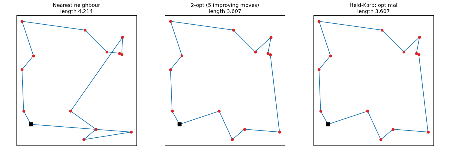
nearest_neighbor length 4.2137 (16.82% above optimal)
two_opt          length 3.6069 ( 0.00% above optimal)
held_karp        length 3.6069 ( 0.00% above optimal)
Held-Karp took 0.05 s

How the exact algorithm scales

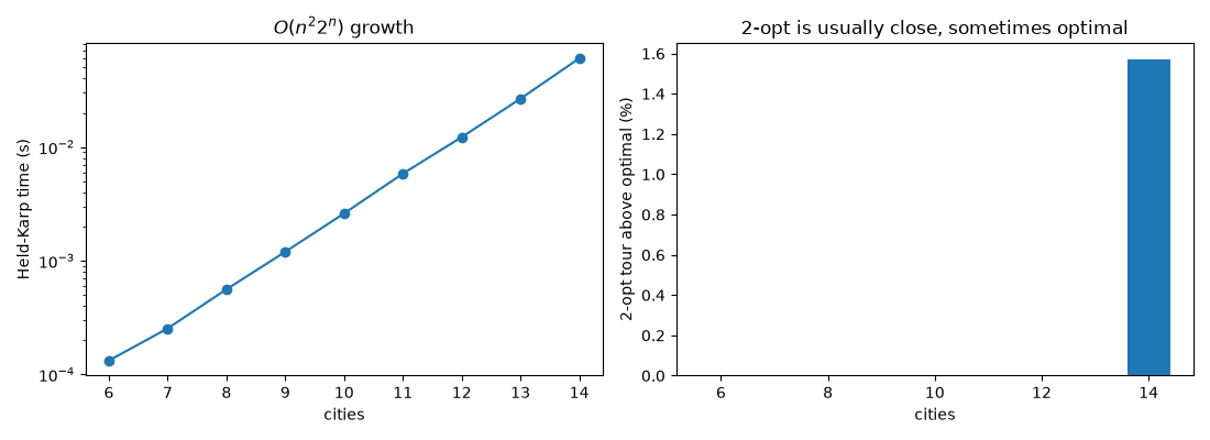
Each extra city roughly doubles Held-Karp’s work, which is why exact methods are reserved for small instances (or for clever branch-and-cut codes such as Concorde), and 2-opt for everything else.

sizes = list(range(6, 15))
times, gaps = [], []
for k in sizes:
    d = distance_matrix(np.random.default_rng(k).uniform(size=(k, 2)))
    t0 = time.perf_counter()
    best = tsp_held_karp(d).length
    times.append(time.perf_counter() - t0)
    gaps.append(100 * (tsp_two_opt(d).length / best - 1))

fig, (ax0, ax1) = plt.subplots(1, 2, figsize=(11, 4))
ax0.semilogy(sizes, times, "o-")
ax0.set_xlabel("cities")
ax0.set_ylabel("Held-Karp time (s)")
ax0.set_title(r"$O(n^2 2^n)$ growth")
ax1.bar(sizes, gaps)
ax1.set_xlabel("cities")
ax1.set_ylabel("2-opt tour above optimal (%)")
ax1.set_title("2-opt is usually close, sometimes optimal")
fig.tight_layout()

plt.show()