Godunov’s method: capturing shocks without oscillations

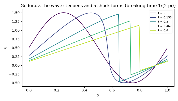
In inviscid Burgers’ equation \(u_t + (u^2/2)_x = 0\), faster fluid overtakes slower fluid and smooth data steepens into a shock. Sergei Godunov (1959) computed the flux between neighboring cells from the exact solution of the Riemann problem they pose. The result is a conservative, monotone scheme that moves shocks at the right speed without spurious wiggles. He also proved that no linear scheme can be both monotone and better than first order, which is why second-order Lax-Wendroff oscillates. This script shows a sine wave breaking into a shock, then compares three schemes on a Riemann problem.

import matplotlib.pyplot as plt
import numpy as np

from mathematicskit.pde import BurgersConservationLaw1D, burgers_riemann_solution, total_variation
from mathematicskit.pde.visualizers import plot_snapshots

A smooth wave breaks into a shock

wave = BurgersConservationLaw1D(lambda x: 0.5 + np.sin(2 * np.pi * x), n=400, bc="periodic")
sol = wave.solve(0.6, dt=0.5 * wave.dx / 1.5, save_every=40)
fig1, ax1 = plt.subplots(figsize=(7, 4))
plot_snapshots(sol, n_snapshots=5, ax=ax1)
ax1.set_title("Godunov: the wave steepens and a shock forms (breaking time 1/(2 pi))")
fig1.tight_layout()

The Riemann problem: shock and rarefaction

u0 = lambda x: np.where(x < -0.3, -0.5, np.where(x < 0.3, 1.0, 0.0))  # a rarefaction, then a shock
law = BurgersConservationLaw1D(u0, x_range=(-1.0, 1.0), n=200)
fig2, ax2 = plt.subplots(figsize=(7, 4))
xs = np.linspace(-1, 1, 1000)
t = 0.6
exact = np.where(xs < 0.0, burgers_riemann_solution(-0.5, 1.0, xs, t, x0=-0.3), burgers_riemann_solution(1.0, 0.0, xs, t, x0=0.3))
ax2.plot(xs, exact, color="black", lw=2, label="exact entropy solution")
for scheme, style in (("godunov", "o"), ("lax_friedrichs", "s"), ("lax_wendroff", "^")):
    s = law.solve(t, dt=0.8 * law.dx, scheme=scheme)
    ax2.plot(s.x, s.final, style, ms=3, label=scheme)
    print(f"{scheme:>15}: max u = {s.final.max():.3f}, total variation {total_variation(law.u0):.2f} -> {total_variation(s.final):.2f}")
ax2.set_xlabel("$x$")
ax2.set_title("Only Godunov is both sharp and free of overshoots")
ax2.legend(fontsize=8)
fig2.tight_layout()

plt.show()

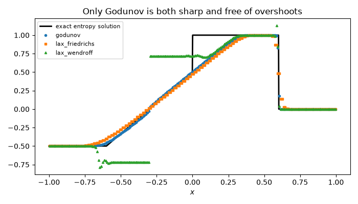
       godunov: max u = 1.000, total variation 2.50 -> 2.50
lax_friedrichs: max u = 1.000, total variation 2.50 -> 2.50
  lax_wendroff: max u = 1.129, total variation 2.50 -> 3.53