Crank-Nicolson: large, stable, second-order heat steps

John Crank and Phyllis Nicolson (1947) averaged the explicit and implicit heat-equation updates. The result is unconditionally stable, like backward Euler, and second-order accurate in time, unlike it. This script shows explicit FTCS blowing up just past its limit \(r = \alpha\Delta t/\Delta x^2 = 1/2\), Crank-Nicolson staying bounded at steps 160 times larger (though not accurate there), and the time-convergence orders that separate Crank-Nicolson from backward Euler.

import matplotlib.pyplot as plt
import numpy as np

from mathematicskit.pde import HeatEquation1D

heat = HeatEquation1D(lambda x: np.sin(np.pi * x) + 0.3 * np.sin(7 * np.pi * x), n=41)
exact = np.sin(np.pi * heat.x) * np.exp(-(np.pi**2) * 0.1) + 0.3 * np.sin(7 * np.pi * heat.x) * np.exp(-49 * np.pi**2 * 0.1)

Explicit FTCS needs r <= 1/2

fig1, ax1 = plt.subplots(figsize=(7, 4))
for r, color in ((0.45, "tab:blue"), (0.55, "tab:red")):
    sol = heat.solve_theta(0.1, dt=r * heat.dx**2, theta=0.0)
    print(f"FTCS r = {r}: stable = {sol.extra['stability'].stable}, max |u| = {np.max(np.abs(sol.final)):.3g}")
    ax1.plot(sol.x, np.clip(sol.final, -1, 1), color=color, label=f"FTCS, r = {r}")
ax1.plot(heat.x, exact, "k--", label="exact")
ax1.set_title("Explicit FTCS just below and just above its stability limit")
ax1.set_xlabel("$x$")
ax1.legend(fontsize=8)
fig1.tight_layout()

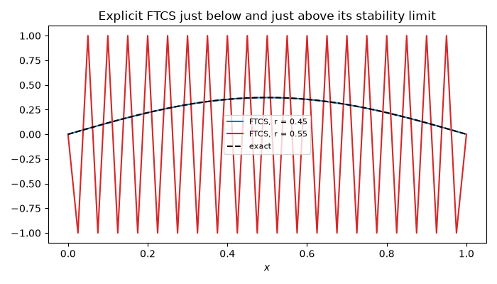
FTCS r = 0.45: stable = True, max |u| = 0.372
FTCS r = 0.55: stable = False, max |u| = 1.11e+06

Crank-Nicolson at r = 80

Stable, but not accurate: at large \(r\) the amplification factor of the fast modes tends to \(-1\), so the \(\sin(7\pi x)\) component flips sign every step instead of decaying. Backward Euler damps it, at the price of only first-order accuracy.

cn = heat.solve_theta(0.1, dt=0.05, theta=0.5)
be = heat.solve_theta(0.1, dt=0.05, theta=1.0)
print(f"Crank-Nicolson r = {cn.extra['stability'].number:.0f}: bounded = {np.max(np.abs(cn.final)) <= 1.3}, max error = {np.max(np.abs(cn.final - exact)):.2e}")
print(f"backward Euler r = {be.extra['stability'].number:.0f}: max error = {np.max(np.abs(be.final - exact)):.2e}")

Crank-Nicolson r = 80: bounded = True, max error = 2.21e-01
backward Euler r = 80: max error = 7.53e-02

Second order in time versus first

Against the exact decay of the semi-discrete system (so only the time error remains), halving \(\Delta t\) quarters the Crank-Nicolson error but only halves the backward-Euler error.

fine = HeatEquation1D(lambda x: np.sin(np.pi * x), n=101)
lam = -4.0 / fine.dx**2 * np.sin(np.pi * fine.dx / 2) ** 2
semi_exact = np.sin(np.pi * fine.x) * np.exp(lam * 0.1)
dts = np.array([0.02, 0.01, 0.005, 0.0025, 0.00125])
fig2, ax2 = plt.subplots(figsize=(6, 4))
for theta, label in ((0.5, "Crank-Nicolson"), (1.0, "backward Euler")):
    errors = [np.max(np.abs(fine.solve_theta(0.1, dt, theta=theta).final - semi_exact)) for dt in dts]
    ax2.loglog(dts, errors, "o-", label=label)
    print(f"{label}: observed order {np.polyfit(np.log(dts), np.log(errors), 1)[0]:.2f}")
ax2.set_xlabel(r"$\Delta t$")
ax2.set_ylabel("max error")
ax2.set_title("Time-convergence of the theta-method")
ax2.legend()
fig2.tight_layout()

plt.show()

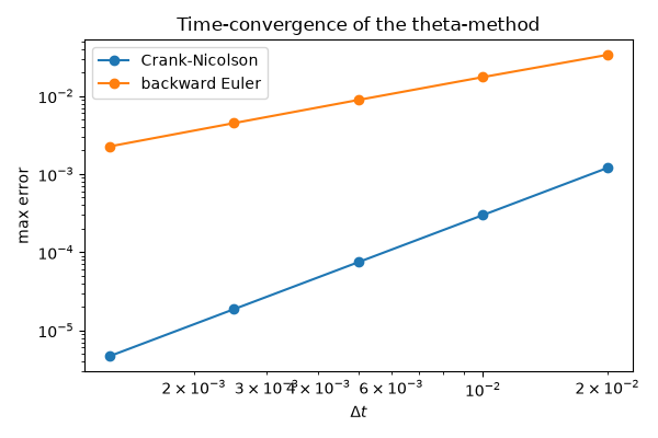
Crank-Nicolson: observed order 2.00
backward Euler: observed order 0.97