The method of lines: a hot plate as a system of ODEs

The method of lines discretizes only space. On a grid, the 2D heat equation \(u_t = u_{xx} + u_{yy}\) becomes one ODE per interior point, \(dU/dt = L U\), which any ODE integrator can then advance. Here that integrator is mathematicskit.integrators.rk4_integrate() (the same one mathematicskit.ode_dynamics uses) and, for comparison, the adaptive dopri5_integrate(). The ODE system is stiff, so RK4’s stable step shrinks like \(\Delta x^2\).

import matplotlib.pyplot as plt
import numpy as np

from mathematicskit.pde import HeatEquation2D
from mathematicskit.pde.visualizers import plot_field_2d


def hot_square(X, Y):
    return np.where((np.abs(X - 0.5) < 0.2) & (np.abs(Y - 0.5) < 0.2), 1.0, 0.0)


heat = HeatEquation2D(hot_square, n=(41, 41))
print(f"ODE system size: {heat.state0.size} unknowns (one per interior grid point)")
print(f"RK4 stable step on this grid: dt <= {heat.max_stable_dt('rk4'):.2e}")

ODE system size: 1521 unknowns (one per interior grid point)
RK4 stable step on this grid: dt <= 2.18e-04

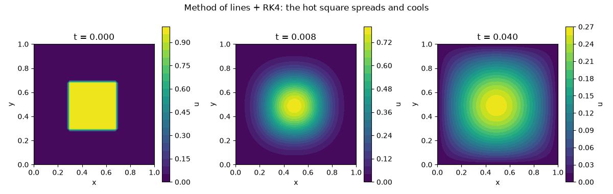
Integrate the semi-discrete system with RK4

sol = heat.solve(0.04, dt=0.9 * heat.max_stable_dt("rk4"), save_every=40)
fig, axes = plt.subplots(1, 3, figsize=(12, 3.8))
for ax, t in zip(axes, (0.0, 0.01, 0.04), strict=False):
    k = int(np.argmin(np.abs(sol.t - t)))
    plot_field_2d(sol, time_index=k, ax=ax)
    ax.set_title(f"t = {sol.t[k]:.3f}")
fig.suptitle("Method of lines + RK4: the hot square spreads and cools")
fig.tight_layout()

An adaptive integrator agrees

adaptive = heat.solve(0.04, method="dopri5", rtol=1e-6, atol=1e-9)
print(f"dopri5 accepted steps: {len(adaptive.t) - 1}")
print(f"max |RK4 - dopri5| at t = 0.04: {np.max(np.abs(sol.final - adaptive.final)):.2e}")

plt.show()

dopri5 accepted steps: 170
max |RK4 - dopri5| at t = 0.04: 3.68e-08