Chebyshev collocation: spectral accuracy without periodicity

Fourier methods need periodic problems. Gottlieb and Orszag’s 1977 monograph set out the theory of the non-periodic alternative: collocate at the Chebyshev points \(x_k = -\cos(k\pi/N)\). These points cluster at the ends and so avoid the Runge phenomenon. This script solves the boundary-value problem \(u'' = f\) with Chebyshev collocation and with second-order finite differences, and watches the Chebyshev error fall geometrically while the finite-difference error only falls like \(N^{-2}\). It closes with a 2D Poisson problem on a square.

import matplotlib.pyplot as plt
import numpy as np

from mathematicskit.pde import chebyshev_poisson_1d, chebyshev_poisson_2d, solve_poisson_1d
from mathematicskit.pde.visualizers import plot_field_2d


def exact(x):
    return np.exp(x) * np.sin(3 * x)


def source(x):
    return np.exp(x) * (-8 * np.sin(3 * x) + 6 * np.cos(3 * x))

Geometric versus algebraic convergence

ns = np.arange(6, 41, 2)
cheb_err, fd_err = [], []
for n in ns:
    c = chebyshev_poisson_1d(source, n=n, ua=exact(-1.0), ub=exact(1.0))
    d = solve_poisson_1d(source, -1.0, 1.0, n, exact(-1.0), exact(1.0))
    cheb_err.append(np.max(np.abs(c.u - exact(c.x))))
    fd_err.append(np.max(np.abs(d.u - exact(d.x))))
fig1, ax1 = plt.subplots(figsize=(6, 4))
ax1.semilogy(ns, np.maximum(cheb_err, 1e-17), "o-", label="Chebyshev collocation")
ax1.semilogy(ns, fd_err, "s-", label="finite differences")
ax1.set_xlabel("grid points $N$")
ax1.set_ylabel("max error")
ax1.set_title(r"$u'' = f$ on $[-1, 1]$")
ax1.legend()
fig1.tight_layout()
print(f"N = 20: Chebyshev error {cheb_err[7]:.1e}, finite-difference error {fd_err[7]:.1e}")

N = 20: Chebyshev error 6.7e-15, finite-difference error 1.6e-02

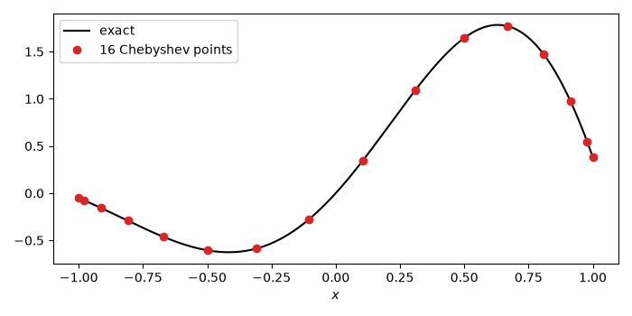
The points cluster at the boundary

c = chebyshev_poisson_1d(source, n=16, ua=exact(-1.0), ub=exact(1.0))
fig2, ax2 = plt.subplots(figsize=(7, 3.5))
x = np.linspace(-1, 1, 400)
ax2.plot(x, exact(x), color="black", label="exact")
ax2.plot(c.x, c.u, "o", color="tab:red", label="16 Chebyshev points")
ax2.set_xlabel("$x$")
ax2.legend()
fig2.tight_layout()

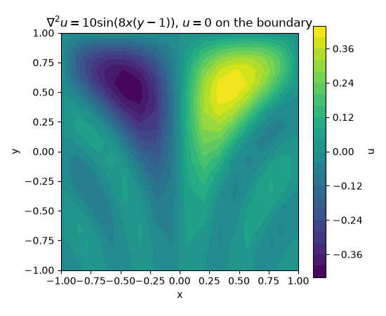
A 2D Poisson problem on a square

sol = chebyshev_poisson_2d(lambda X, Y: 10 * np.sin(8 * X * (Y - 1)), n=24)
fig3, ax3 = plt.subplots(figsize=(5.5, 4.5))
plot_field_2d(sol, ax=ax3, levels=25)
ax3.set_title(r"$\nabla^2 u = 10 \sin(8x(y-1))$, $u = 0$ on the boundary")
fig3.tight_layout()

plt.show()