Burgers’ equation and the Hopf-Cole transformation

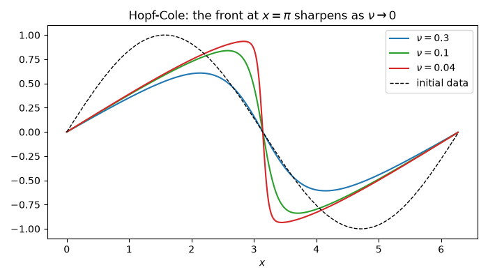
J. M. Burgers (1948) proposed viscous Burgers’ equation as the simplest model of nonlinear steepening balanced by viscosity. Eberhard Hopf (1950) and Julian Cole (1951) independently found that the substitution \(u = -2\nu\,\varphi_x/\varphi\) turns the nonlinear viscous Burgers’ equation \(u_t + u u_x = \nu u_{xx}\) into the linear heat equation \(\varphi_t = \nu\varphi_{xx}\). A nonlinear PDE with shock-like fronts thus has an exact solution. This script uses it to watch a sine wave form a viscous shock whose width shrinks with \(\nu\), and to verify the pseudo-spectral Burgers solver to near machine precision.

import matplotlib.pyplot as plt
import numpy as np

from mathematicskit.pde import BurgersEquation1D, burgers_cole_hopf_solution

Viscous shocks, exactly

fig1, ax1 = plt.subplots(figsize=(7, 4))
for nu, color in ((0.3, "tab:blue"), (0.1, "tab:green"), (0.04, "tab:red")):
    x, u = burgers_cole_hopf_solution(np.sin, t=1.5, nu=nu, n=512)
    ax1.plot(x, u, color=color, label=rf"$\nu = {nu}$")
ax1.plot(x, np.sin(x), "k--", lw=1, label="initial data")
ax1.set_xlabel("$x$")
ax1.set_title(r"Hopf-Cole: the front at $x = \pi$ sharpens as $\nu \to 0$")
ax1.legend()
fig1.tight_layout()

An exact benchmark for the numerical solver

nu, t = 0.1, 1.0
for n in (32, 64, 128):
    x, exact = burgers_cole_hopf_solution(np.sin, t=t, nu=nu, n=n)
    numerical = BurgersEquation1D(np.sin, n=n, nu=nu).solve(t, dt=1e-3).final
    print(f"n = {n:3d}: max |pseudo-spectral - Hopf-Cole| = {np.max(np.abs(numerical - exact)):.1e}")

plt.show()

n =  32: max |pseudo-spectral - Hopf-Cole| = 1.3e-04
n =  64: max |pseudo-spectral - Hopf-Cole| = 4.5e-08
n = 128: max |pseudo-spectral - Hopf-Cole| = 6.5e-13