Kolmogorov’s axioms: events as sets, probability as a measure

Kolmogorov (1933) defined a probability space \((\Omega, \mathcal F, P)\): a sample space \(\Omega\), a collection \(\mathcal F\) of events (subsets of \(\Omega\)), and a measure \(P\) satisfying

1. non-negativity – \(P(E) \geq 0\) for every event \(E\);

2. normalization – \(P(\Omega) = 1\);

3. countable additivity – \(P(\bigcup_i E_i) = \sum_i P(E_i)\) for pairwise disjoint events.

Conditional probability \(P(A \mid B) = P(A \cap B)/P(B)\) and independence \(P(A \cap B) = P(A)P(B)\) are then definitions built on top. This example checks the axioms on a finite space (two dice) and on the pmf/pdf/cdf of this package’s distributions.

import itertools
from fractions import Fraction

import matplotlib.pyplot as plt
import numpy as np
from scipy import integrate

from mathematicskit.probability import Binomial, Gamma, Normal, Poisson

A finite probability space: two fair dice

Every event is a set of outcomes, and \(P(E) = |E| / 36\).

omega = frozenset(itertools.product(range(1, 7), repeat=2))


def prob(event):
    return Fraction(len(event), len(omega))


sum_is_7 = frozenset(w for w in omega if sum(w) == 7)
first_even = frozenset(w for w in omega if w[0] % 2 == 0)
doubles = frozenset(w for w in omega if w[0] == w[1])

print("axiom 1, P(E) >= 0 for events tested:", all(prob(e) >= 0 for e in (sum_is_7, first_even, doubles, frozenset())))
print("axiom 2, P(Omega) =", prob(omega))
print(
    "axiom 3, disjoint {sum=7} and {doubles}:",
    f"P(union) = {prob(sum_is_7 | doubles)} = {prob(sum_is_7)} + {prob(doubles)}",
)
print(f"derived: P(sum=7 | first even) = {prob(sum_is_7 & first_even) / prob(first_even)}")
print("derived: {sum=7} and {first even} independent:", prob(sum_is_7 & first_even) == prob(sum_is_7) * prob(first_even))

axiom 1, P(E) >= 0 for events tested: True
axiom 2, P(Omega) = 1
axiom 3, disjoint {sum=7} and {doubles}: P(union) = 1/3 = 1/6 + 1/6
derived: P(sum=7 | first even) = 1/6
derived: {sum=7} and {first even} independent: True

Probability as a measure on the real line

A distribution assigns \(P((a, b]) = F(b) - F(a)\). The pmf sums to one and the pdf integrates to one (normalization), and the measure of a union of disjoint intervals is the sum of their measures.

poisson = Poisson(mu=3.0)
ks = np.arange(0, 200)
print(f"Poisson: min pmf = {poisson.pmf(ks).min():.1e} >= 0, sum of pmf over N = {poisson.pmf(ks).sum():.12f}")
print(f"Binomial(10, 0.4): sum of pmf = {Binomial(n=10, p=0.4).pmf(np.arange(11)).sum():.12f}")
for dist in (Normal(mu=0.0, sigma=1.0), Gamma(shape=2.0, rate=1.5)):
    lower = -np.inf if isinstance(dist, Normal) else 0.0
    total, _ = integrate.quad(dist.pdf, lower, np.inf)
    print(f"{type(dist).__name__}: integral of pdf = {total:.10f}")

normal = Normal(mu=0.0, sigma=1.0)
cuts = [-2.0, -0.5, 0.7, 1.8]
pieces = [normal.cdf(b) - normal.cdf(a) for a, b in zip(cuts[:-1], cuts[1:])]
print(f"additivity: P((-2, 1.8]) = {normal.cdf(1.8) - normal.cdf(-2.0):.6f}, sum of disjoint pieces = {sum(pieces):.6f}")

Poisson: min pmf = 1.1e-279 >= 0, sum of pmf over N = 1.000000000000
Binomial(10, 0.4): sum of pmf = 1.000000000000
Normal: integral of pdf = 1.0000000000
Gamma: integral of pdf = 1.0000000000
additivity: P((-2, 1.8]) = 0.941320, sum of disjoint pieces = 0.941320

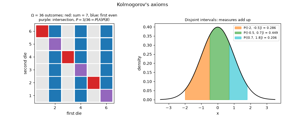
Picture: events are sets, probabilities are areas

fig, (ax_dice, ax_line) = plt.subplots(1, 2, figsize=(10, 4.2))
for i, j in omega:
    in_a, in_b = (i, j) in sum_is_7, (i, j) in first_even
    color = "tab:purple" if in_a and in_b else "tab:red" if in_a else "tab:blue" if in_b else "0.9"
    ax_dice.add_patch(plt.Rectangle((i - 0.45, j - 0.45), 0.9, 0.9, color=color))
ax_dice.set_xlim(0.4, 6.6)
ax_dice.set_ylim(0.4, 6.6)
ax_dice.set_aspect("equal")
ax_dice.set_xlabel("first die")
ax_dice.set_ylabel("second die")
ax_dice.set_title(r"$\Omega$ = 36 outcomes; red: sum = 7, blue: first even" "\npurple: intersection, $P = 3/36 = P(A)P(B)$", fontsize=9)

xs = np.linspace(-3.5, 3.5, 400)
ax_line.plot(xs, normal.pdf(xs), "k")
for (a, b), piece, color in zip(zip(cuts[:-1], cuts[1:]), pieces, ("tab:orange", "tab:green", "tab:cyan")):
    mask = (xs > a) & (xs <= b)
    ax_line.fill_between(xs[mask], normal.pdf(xs[mask]), color=color, alpha=0.6, label=f"P(({a:g}, {b:g}]) = {piece:.3f}")
ax_line.set_xlabel("x")
ax_line.set_ylabel("density")
ax_line.set_title("Disjoint intervals: measures add up", fontsize=9)
ax_line.legend(fontsize=8)
fig.suptitle("Kolmogorov's axioms")
fig.tight_layout()