Bayes’s problem: learning a probability from data

Starting from Bayes’s uniform prior, the posterior for an unknown success probability \(p\) after \(k\) successes in \(n\) trials is \(\mathrm{Beta}(k+1, n-k+1)\). It narrows around the true value as data accumulate, and its mean is Laplace’s rule of succession \((k+1)/(n+2)\).

import matplotlib.pyplot as plt
import numpy as np

from mathematicskit.probability import beta_binomial_posterior, rule_of_succession

Posteriors after more and more trials

p_true = 0.3
rng = np.random.default_rng(0)
flips = rng.random(1000) < p_true
x = np.linspace(0.0, 1.0, 500)

fig, ax = plt.subplots()
for n in (0, 5, 20, 100, 1000):
    k = int(flips[:n].sum())
    post = beta_binomial_posterior(k, n)
    lo, hi = post.ppf([0.025, 0.975])
    print(f"n={n:>4}, k={k:>3}: next-success probability {rule_of_succession(k, n):.4f}, 95% interval [{lo:.3f}, {hi:.3f}]")
    ax.plot(x, post.pdf(x), label=f"n = {n}")
ax.axvline(p_true, color="0.3", ls="--", label="true p")
ax.set_xlabel("p")
ax.set_ylabel("posterior density")
ax.legend()
ax.set_title("Bayes (1763): Beta posteriors from a uniform prior")

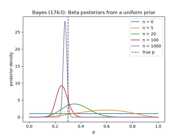
n=   0, k=  0: next-success probability 0.5000, 95% interval [0.025, 0.975]
n=   5, k=  3: next-success probability 0.5714, 95% interval [0.223, 0.882]
n=  20, k=  7: next-success probability 0.3636, 95% interval [0.181, 0.570]
n= 100, k= 25: next-success probability 0.2549, 95% interval [0.176, 0.343]
n=1000, k=277: next-success probability 0.2774, 95% interval [0.250, 0.306]

Text(0.5, 1.0, 'Bayes (1763): Beta posteriors from a uniform prior')