The gamma distribution generalizes the exponential

A Gamma(shape=1, rate) distribution is exactly an Exponential(rate); increasing the shape parameter builds up a sum of exponentials.

import numpy as np

from mathematicskit.probability import Exponential, Gamma, Normal
from mathematicskit.probability.visualizers.plots import plot_distribution

Gamma(1, rate) matches Exponential(rate) exactly

rate = 2.0
gamma = Gamma(shape=1.0, rate=rate)
exponential = Exponential(rate=rate)
xs = np.linspace(0.01, 3.0, 50)
print("max |gamma(1,r) - exponential(r)| pdf difference:", np.max(np.abs(gamma.pdf(xs) - exponential.pdf(xs))))

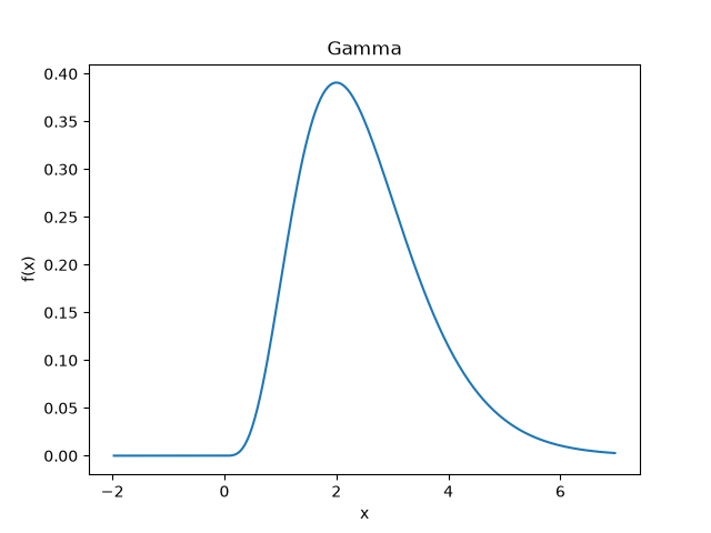
plot_distribution(Gamma(shape=5.0, rate=2.0))

max |gamma(1,r) - exponential(r)| pdf difference: 0.0

<Axes: title={'center': 'Gamma'}, xlabel='x', ylabel='f(x)'>

The normal distribution and its MGF

normal = Normal(mu=0.0, sigma=1.0)
print("normal MGF at t=1:", normal.mgf(1.0), "expected exp(0.5):", np.exp(0.5))
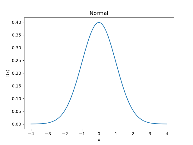
plot_distribution(normal)

normal MGF at t=1: 1.6487212707001282 expected exp(0.5): 1.6487212707001282

<Axes: title={'center': 'Normal'}, xlabel='x', ylabel='f(x)'>