Poisson’s law of rare events: the binomial limit

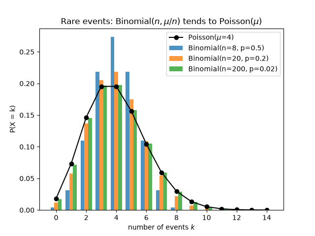
Many independent trials, each with a tiny chance of success, produce a number of successes that follows a Poisson distribution. Poisson (1837) obtained it as the limit of \(\mathrm{Binomial}(n, p)\) with \(n \to \infty\), \(p \to 0\) and the mean \(np = \mu\) held fixed:

\[\binom{n}{k} p^k (1-p)^{n-k} \;\longrightarrow\; e^{-\mu}\frac{\mu^k}{k!}.\]

import matplotlib.pyplot as plt
import numpy as np

from mathematicskit.probability import Binomial, Poisson

mu = 4.0
poisson = Poisson(mu=mu)
ks = np.arange(0, 15)

Binomial PMFs approach the Poisson PMF as events become rarer

fig, ax = plt.subplots()
width = 0.25
for offset, n in zip((-width, 0.0, width), (8, 20, 200)):
    ax.bar(ks + offset, Binomial(n=n, p=mu / n).pmf(ks), width=width, alpha=0.8, label=f"Binomial(n={n}, p={mu / n:.3g})")
ax.plot(ks, poisson.pmf(ks), "ko-", label=rf"Poisson($\mu$={mu:g})")
ax.set_xlabel("number of events $k$")
ax.set_ylabel("P(X = k)")
ax.set_title(r"Rare events: Binomial$(n, \mu/n)$ tends to Poisson$(\mu)$")
ax.legend()

<matplotlib.legend.Legend object at 0x11a99cec0>

The largest PMF gap shrinks like 1/n

ns = np.array([10, 30, 100, 300, 1000, 3000, 10000])
gaps = np.array([np.max(np.abs(Binomial(n=int(n), p=mu / n).pmf(ks) - poisson.pmf(ks))) for n in ns])
for n, gap in zip(ns, gaps):
    print(f"n={n:>6}: max |binomial - poisson| = {gap:.2e}")

fig, ax = plt.subplots()
ax.loglog(ns, gaps, "o-", label="max PMF difference")
ax.loglog(ns, gaps[0] * ns[0] / ns, "k--", label=r"$\propto 1/n$")
ax.set_xlabel("number of trials $n$ (with $np = 4$)")
ax.set_ylabel("max |Binomial - Poisson|")
ax.set_title("Poisson limit theorem")
ax.legend()

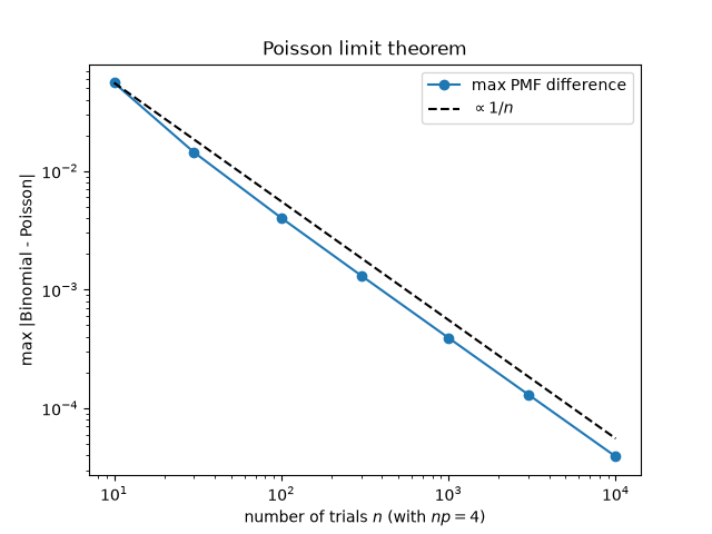
n=    10: max |binomial - poisson| = 5.55e-02
n=    30: max |binomial - poisson| = 1.44e-02
n=   100: max |binomial - poisson| = 4.02e-03
n=   300: max |binomial - poisson| = 1.31e-03
n=  1000: max |binomial - poisson| = 3.92e-04
n=  3000: max |binomial - poisson| = 1.30e-04
n= 10000: max |binomial - poisson| = 3.91e-05

<matplotlib.legend.Legend object at 0x11ce352b0>

A rare-event count: simulated arrivals

100000 independent units, each failing with probability 4e-5 in a day: the daily count of failures is Poisson with mean 4.

counts = Binomial(n=100000, p=4e-5).sample(size=20000, seed=0)
print(f"mean daily failures = {counts.mean():.3f}, variance = {counts.var():.3f} (Poisson: both = {mu})")
print(f"P(no failures): simulated {np.mean(counts == 0):.4f}, Poisson e^-4 = {poisson.pmf(0):.4f}")

mean daily failures = 3.971, variance = 4.045 (Poisson: both = 4.0)
P(no failures): simulated 0.0202, Poisson e^-4 = 0.0183