Kolmogorov’s equations: a continuous-time Markov chain

A machine is working (0), degraded (1), or broken (2), jumping between states at the rates in the generator \(Q\). The transition matrix \(P(t) = e^{tQ}\) solves Kolmogorov’s forward and backward equations and relaxes to the stationary distribution \(\pi\), the solution of \(\pi Q = 0\).

import matplotlib.pyplot as plt
import numpy as np

from mathematicskit.probability import ctmc_stationary_distribution, ctmc_transition_matrix

Q = np.array(
    [
        [-0.5, 0.4, 0.1],
        [0.0, -1.0, 1.0],
        [2.0, 0.0, -2.0],
    ]
)

State probabilities starting from “working”

times = np.linspace(0.0, 8.0, 200)
probs = np.array([ctmc_transition_matrix(Q, t)[0] for t in times])
pi = ctmc_stationary_distribution(Q)
print(f"stationary distribution: {pi.round(4)}")

fig, ax = plt.subplots()
for j, name in enumerate(["working", "degraded", "broken"]):
    (line,) = ax.plot(times, probs[:, j], label=name)
    ax.axhline(pi[j], color=line.get_color(), ls=":")
ax.set_xlabel("t")
ax.set_ylabel(r"$P_{0j}(t)$")
ax.legend()
ax.set_title(r"$P(t) = e^{tQ}$ converging to $\pi$")

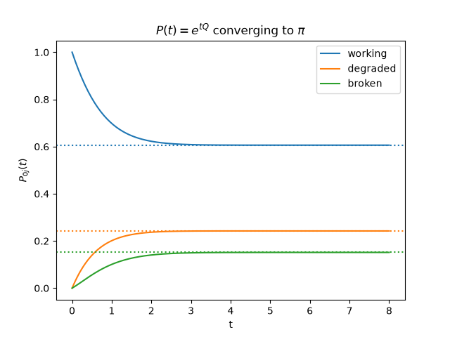
stationary distribution: [0.6061 0.2424 0.1515]

Text(0.5, 1.0, '$P(t) = e^{tQ}$ converging to $\\pi$')