Markov chain Monte Carlo: Metropolis-Hastings and the Gibbs sampler

Hastings (1970) generalized the 1953 Metropolis algorithm into a recipe for sampling any density \(\pi\) known only up to a constant: propose \(y \sim q(\cdot \mid x)\), accept with probability \(\min\bigl(1, \pi(y)q(x \mid y) / \pi(x)q(y \mid x)\bigr)\). Geman and Geman (1984) sampled images one pixel at a time from its conditional distribution given the rest: the Gibbs sampler.

The target here is a banana-shaped density (a Gaussian twisted by \(y \mapsto y - b x^2\)), whose normalizing constant never appears in either algorithm. Its exact moments are known: \(E[x] = 0\), \(E[y] = b\), \(\operatorname{Var}x = 1\) and \(\operatorname{Var}y = 1 + 2b^2\).

import matplotlib.pyplot as plt
import numpy as np

from mathematicskit.probability import chain_effective_sample_size, gibbs_sampler, metropolis_hastings

b = 1.0


def log_banana(z):
    x, y = z
    return -0.5 * x**2 - 0.5 * (y - b * x**2) ** 2

Metropolis-Hastings: the step size trades acceptance against mixing

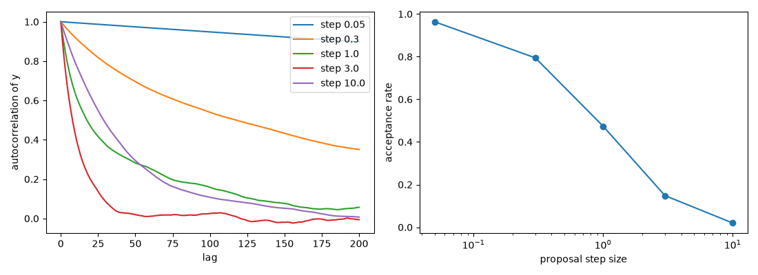
Tiny steps are almost always accepted but crawl; huge steps are almost always rejected. The effective sample size of \(y\) (how many independent draws the correlated chain is worth, see chain_effective_sample_size()) peaks in between.

scales = [0.05, 0.3, 1.0, 3.0, 10.0]
runs = {s: metropolis_hastings(log_banana, [0.0, 0.0], n_samples=50000, proposal_scale=s, burn_in=1000, seed=1) for s in scales}
for s, run in runs.items():
    ess = chain_effective_sample_size(run.samples[:, 1])
    print(f"step {s:5.2f}: acceptance {run.acceptance_rate:.2f}, effective sample size of y = {ess:7.0f}")

best = runs[3.0]
print(f"MH mean  = {best.samples.mean(axis=0).round(2)} (exact [0, {b}])")
print(f"MH var   = {best.samples.var(axis=0).round(2)} (exact [1, {1 + 2 * b**2}])")

step  0.05: acceptance 0.96, effective sample size of y =      16
step  0.30: acceptance 0.79, effective sample size of y =     120
step  1.00: acceptance 0.47, effective sample size of y =     538
step  3.00: acceptance 0.15, effective sample size of y =    1945
step 10.00: acceptance 0.02, effective sample size of y =     571
MH mean  = [0.04 0.98] (exact [0, 1.0])
MH var   = [0.97 2.81] (exact [1, 3.0])

The Gibbs sampler: exact conditionals, no rejections

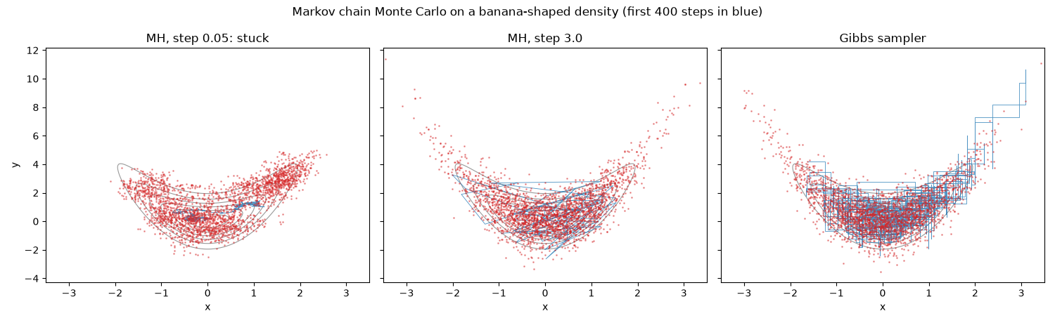
For this density both full conditionals are Gaussian: \(y \mid x \sim \mathcal N(b x^2, 1)\), and, writing the exponent in \(x\), \(x \mid y\) is a quartic that we sample with one inner Metropolis step (a “Metropolis-within-Gibbs” update, still a valid move for \(\pi\)). Each sweep updates one coordinate at a time, so the chain moves in axis-parallel steps.

def draw_x(z, rng):
    x, y = z
    proposal = x + 0.8 * rng.standard_normal()
    log_ratio = log_banana((proposal, y)) - log_banana((x, y))
    return proposal if np.log(rng.uniform()) < log_ratio else x


def draw_y(z, rng):
    return b * z[0] ** 2 + rng.standard_normal()


gibbs = gibbs_sampler([draw_x, draw_y], [0.0, 0.0], n_samples=50000, burn_in=1000, seed=2)
print(f"Gibbs mean = {gibbs.samples.mean(axis=0).round(2)}, var = {gibbs.samples.var(axis=0).round(2)}")

Gibbs mean = [-0.02  0.98], var = [0.98 2.77]

Chains on the target

grid_x, grid_y = np.meshgrid(np.linspace(-3.5, 3.5, 200), np.linspace(-2.5, 9, 200))
density = np.exp(log_banana((grid_x, grid_y)))

fig, axes = plt.subplots(1, 3, figsize=(15, 4.6), sharey=True)
for ax, (label, chain) in zip(axes, [("MH, step 0.05: stuck", runs[0.05]), ("MH, step 3.0", runs[3.0]), ("Gibbs sampler", gibbs)], strict=True):
    ax.contour(grid_x, grid_y, density, levels=6, colors="0.6", linewidths=0.8)
    ax.plot(*chain.samples[:400].T, "-", color="tab:blue", lw=0.6, alpha=0.8, drawstyle="steps-post" if "Gibbs" in label else "default")
    ax.plot(*chain.samples[::20].T, ".", color="tab:red", ms=2, alpha=0.4)
    ax.set_title(label)
    ax.set_xlabel("x")
axes[0].set_ylabel("y")
fig.suptitle("Markov chain Monte Carlo on a banana-shaped density (first 400 steps in blue)")
fig.tight_layout()

Autocorrelation and acceptance

fig, (ax0, ax1) = plt.subplots(1, 2, figsize=(11, 4))
for s, run in runs.items():
    y = run.samples[:, 1] - run.samples[:, 1].mean()
    acf = np.correlate(y, y, mode="full")[y.size - 1 : y.size + 200] / (y @ y)
    ax0.plot(acf, label=f"step {s}")
ax0.set_xlabel("lag")
ax0.set_ylabel("autocorrelation of y")
ax0.legend()
ax1.semilogx(scales, [runs[s].acceptance_rate for s in scales], "o-")
ax1.set_xlabel("proposal step size")
ax1.set_ylabel("acceptance rate")
fig.tight_layout()

plt.show()