The Monte Carlo method: estimating an integral by random sampling

Ulam and von Neumann’s idea: replace an exact calculation by an average over random samples. For \(U \sim \mathrm{Uniform}(0, 1)\),

\[\int_0^1 e^x\,dx = E[e^U] \approx \frac1n \sum_{i=1}^n e^{U_i},\]

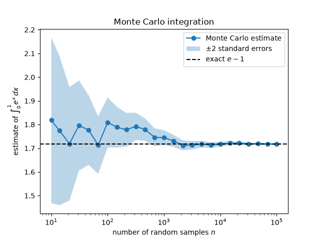
with an error that shrinks like \(1/\sqrt n\) regardless of dimension. The exact value is \(e - 1\). Importance sampling and control variates then reduce the error at the same sample size.

import matplotlib.pyplot as plt
import numpy as np

from mathematicskit.probability.systems.monte_carlo import control_variates_integrate, importance_sampling_integrate, monte_carlo_integrate

exact = np.e - 1.0

Plain Monte Carlo: the estimate converges like 1/sqrt(n)

ns = np.unique(np.logspace(1, 5, 25).astype(int))
estimates = [monte_carlo_integrate(np.exp, 0.0, 1.0, n=int(n), seed=0) for n in ns]
values = np.array([r.estimate for r in estimates])
errors = np.array([r.std_error for r in estimates])

fig, ax = plt.subplots()
ax.semilogx(ns, values, "o-", label="Monte Carlo estimate")
ax.fill_between(ns, values - 2 * errors, values + 2 * errors, alpha=0.3, label=r"$\pm 2$ standard errors")
ax.axhline(exact, color="k", ls="--", label="exact $e - 1$")
ax.set_xlabel("number of random samples $n$")
ax.set_ylabel(r"estimate of $\int_0^1 e^x\,dx$")
ax.set_title("Monte Carlo integration")
ax.legend()

<matplotlib.legend.Legend object at 0x11cf70d70>

Three estimators at the same sample size

n = 20000
plain = monte_carlo_integrate(np.exp, 0.0, 1.0, n=n, seed=0)
print(f"plain:               estimate={plain.estimate:.5f}, std_error={plain.std_error:.5f}")

# importance sampling with q(x) = (1 + x) / 1.5 on [0, 1], drawn by inverting its CDF
importance = importance_sampling_integrate(
    lambda x: np.exp(x) * ((x >= 0.0) & (x <= 1.0)),
    proposal_sampler=lambda rng, size: -1.0 + np.sqrt(1.0 + 3.0 * rng.uniform(size=size)),
    proposal_pdf=lambda x: (1.0 + x) / 1.5,
    n=n,
    seed=0,
)
print(f"importance sampling: estimate={importance.estimate:.5f}, std_error={importance.std_error:.5f}")

# control variate g(x) = x, with E[U] = 0.5 known exactly
cv = control_variates_integrate(np.exp, lambda x: x, control_mean=0.5, a=0.0, b=1.0, n=n, seed=0)
print(f"control variate:     estimate={cv.estimate:.5f}, std_error={cv.std_error:.5f}")

print(f"\nexact value e - 1 = {exact:.5f}")
print(f"variance reduction: importance {(plain.std_error / importance.std_error) ** 2:.1f}x, control variate {(plain.std_error / cv.std_error) ** 2:.1f}x")

plain:               estimate=1.72216, std_error=0.00347
importance sampling: estimate=1.71966, std_error=0.00116
control variate:     estimate=1.71775, std_error=0.00044

exact value e - 1 = 1.71828
variance reduction: importance 9.0x, control variate 60.8x