Itô calculus and the Euler-Maruyama scheme

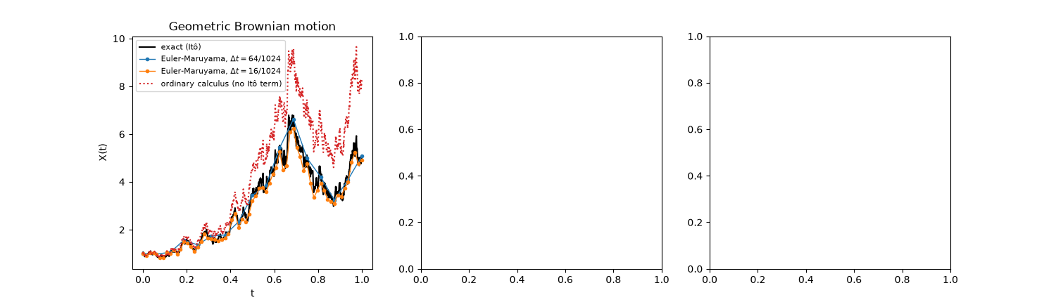
Itô (1944) gave meaning to \(dX = a\,dt + b\,dW\) when \(W\) is Brownian motion, whose paths have no derivative. His chain rule has an extra term: for geometric Brownian motion \(dX = \mu X\,dt + \sigma X\,dW\) it gives

\[X_t = X_0 \exp\!\left(\left(\mu - \tfrac12\sigma^2\right)t + \sigma W_t\right),\]

so the typical path grows at rate \(\mu - \sigma^2/2\), not \(\mu\). Maruyama (1955) proved that the Euler step \(X_{n+1} = X_n + a\Delta t + b\,\Delta W_n\) converges to this solution, with pathwise (strong) error \(O(\Delta t^{1/2})\) and error in expectations (weak) \(O(\Delta t)\).

import matplotlib.pyplot as plt
import numpy as np

from mathematicskit.probability import euler_maruyama, geometric_brownian_motion, ornstein_uhlenbeck

mu, sigma, t_max = 1.0, 1.0, 1.0

One Brownian path, two solutions

The exact solution and Euler-Maruyama share the same Brownian path, so their gap is the scheme’s error alone.

exact = geometric_brownian_motion(mu, sigma, t_max=t_max, n_steps=2**10, n_paths=1, seed=3)
dw_fine = np.diff(exact.wiener, axis=1)

fig, (ax0, ax1, ax2) = plt.subplots(1, 3, figsize=(15, 4.3))
ax0.plot(exact.times, exact.paths[0], "k", lw=1.5, label="exact (Itô)")
for r in (64, 16):
    em = euler_maruyama(lambda x, t: mu * x, lambda x, t: sigma * x, 1.0, t_max, 2**10 // r, dw=dw_fine.reshape(1, -1, r).sum(axis=2))
    ax0.plot(em.times, em.paths[0], "o-", ms=3, lw=1, label=rf"Euler-Maruyama, $\Delta t = {r}/1024$")
naive = np.exp(mu * exact.times + sigma * exact.wiener[0])
ax0.plot(exact.times, naive, ":", color="tab:red", label="ordinary calculus (no Itô term)")
ax0.set_xlabel("t")
ax0.set_ylabel("X(t)")
ax0.set_title("Geometric Brownian motion")
ax0.legend(fontsize=8)

<matplotlib.legend.Legend object at 0x112bcfa10>

Strong order 1/2, weak order 1

many = geometric_brownian_motion(mu, sigma, t_max=t_max, n_steps=2**10, n_paths=4000, seed=4)
dw_many = np.diff(many.wiener, axis=1)
ratios = [8, 16, 32, 64, 128]
dts, strong, weak = [], [], []
for r in ratios:
    em = euler_maruyama(lambda x, t: mu * x, lambda x, t: sigma * x, 1.0, t_max, 2**10 // r, dw=dw_many.reshape(4000, -1, r).sum(axis=2))
    dts.append(t_max * r / 2**10)
    strong.append(np.mean(np.abs(em.paths[:, -1] - many.paths[:, -1])))
    weak.append(abs(em.paths[:, -1].mean() - np.exp(mu * t_max)))
dts = np.array(dts)
strong_slope = np.polyfit(np.log(dts), np.log(strong), 1)[0]
print(f"strong order: {strong_slope:.2f} (theory 0.5)")

ax1.loglog(dts, strong, "o-", label=f"strong error, slope {strong_slope:.2f}")
ax1.loglog(dts, weak, "s-", label="weak error (Monte Carlo noise at small dt)")
ax1.loglog(dts, strong[-1] * np.sqrt(dts / dts[-1]), "k--", lw=0.8, label=r"$\propto \Delta t^{1/2}$")
ax1.loglog(dts, weak[-1] * dts / dts[-1], "k:", lw=0.8, label=r"$\propto \Delta t$")
ax1.set_xlabel(r"$\Delta t$")
ax1.set_ylabel("error at t = 1")
ax1.set_title("Convergence of Euler-Maruyama")
ax1.legend(fontsize=8)

strong order: 0.47 (theory 0.5)

<matplotlib.legend.Legend object at 0x1133d9010>

The Ornstein-Uhlenbeck process relaxes to its stationary law

theta, mean, noise = 2.0, 0.0, 1.0
ou = ornstein_uhlenbeck(theta, mean, noise, x0=3.0, t_max=3.0, n_steps=600, n_paths=5000, seed=5)
t = ou.times
ax2.plot(t, ou.paths[:20].T, lw=0.5, color="tab:blue", alpha=0.5)
expected = mean + (3.0 - mean) * np.exp(-theta * t)
sd = noise * np.sqrt((1 - np.exp(-2 * theta * t)) / (2 * theta))
ax2.plot(t, expected, "k", label="exact mean")
ax2.fill_between(t, expected - 2 * sd, expected + 2 * sd, color="0.8", label=r"exact $\pm 2$ sd")
ax2.set_xlabel("t")
ax2.set_title(r"Ornstein-Uhlenbeck: $dX = -\theta X\,dt + \sigma\,dW$")
ax2.legend(fontsize=8)
fig.tight_layout()

print(f"OU at t = 3: mean {ou.paths[:, -1].mean():.3f} (exact {expected[-1]:.3f}), var {ou.paths[:, -1].var():.3f} (exact {sd[-1] ** 2:.3f})")

plt.show()

OU at t = 3: mean 0.006 (exact 0.007), var 0.250 (exact 0.250)